Report on the Predicting the Productivity of Biochemistry Students

Report on the Predicting the Productivity of Biochemistry Students

Introduction The aim of this report is to model the productivity of biochemistry students. In the report, we measure the productivity by a number of published articles. We hypothesize that there is a relationship between productivity (art) and following covariates: gender (gend), number of publications of mentor (ment), prestige of department (prest), number of kids below age of 5 (kid5), and marital status of a student (mar). Before we begin the analysis, it is important to be aware of the limitations of the dataset. Although the sample of students is relatively big (915 observations), we do not know: If the students were randomly selected within a department? If the departments were randomly selected from different countries/regions? How the prestige of the department was measured? We need to keep these limitations in mind when interpreting the results. Lack of knowledge about (2) might cause lack of generalizability of our model. For the purpose of below analysis, we assume independence (1). Otherwise the below estimators might be biased, meaning that we would not be able to accurately predict the productivity of students.

Exploratory Data Analysis Firstly, we check if all the entries within dataset are correct. Checks include: testing if all variables have the same length, testing the type of particular variables, checking if range is reasonable. None of the observations display obvious errors. Thus, we may proceed to numerical exploratory analysis. We note that the variables mentor, dept, art, and kid5 are numerical variables, with all except dept, which takes values in 1 - 5, taking integer values. The remaining two variables, gender and mar, are categorical, each taking two values. Although kid5 is numeric, it takes only four values (0, 1, 2, and 3), so may also be considered categorical. For convenience, we relabel the levels to more appropriate names - male and female for gender, and no and yes for mar. mentor refers to the number of articles the student’s mentor has published over the last three years, art the number of articles the student has published over the same period. gender refers to the student’s gender, and mar to their marital status. kid5 gives the number of children they have who are aged five or younger, and dept the prestige rating of their department, on a scale of 0 to 5.

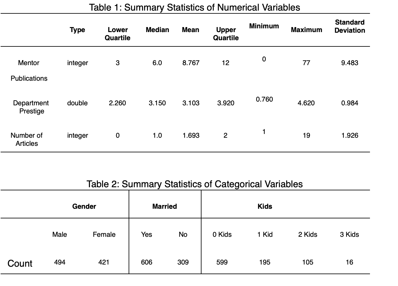
Numerical EDA Table 1 shows, as expected, that the median of articles published by mentors is higher than the median of articles published by PhD students. Standard deviation is lower higher in case of number of articles published by students, in comparison to number of articles published by mentors. It means that there is much higher variability in number of mentor’s publications. Minimum and maximum values of all numerical variables suggest possible outliers in our data. For instance, we may notice that some mentors didn’t publish any articles within analysed time-frame, while one published 77 articles, while the students themselves varied from none to 19. Table 2 presents the summary statistics for categorical data. We notice that our sample is well balanced gender-wise, however there are significantly more married subjects, with almost two thirds of students being married. Similarly, students tend to have either no children, or small amount of children. Just 13% of PhD students have 2 children or more.

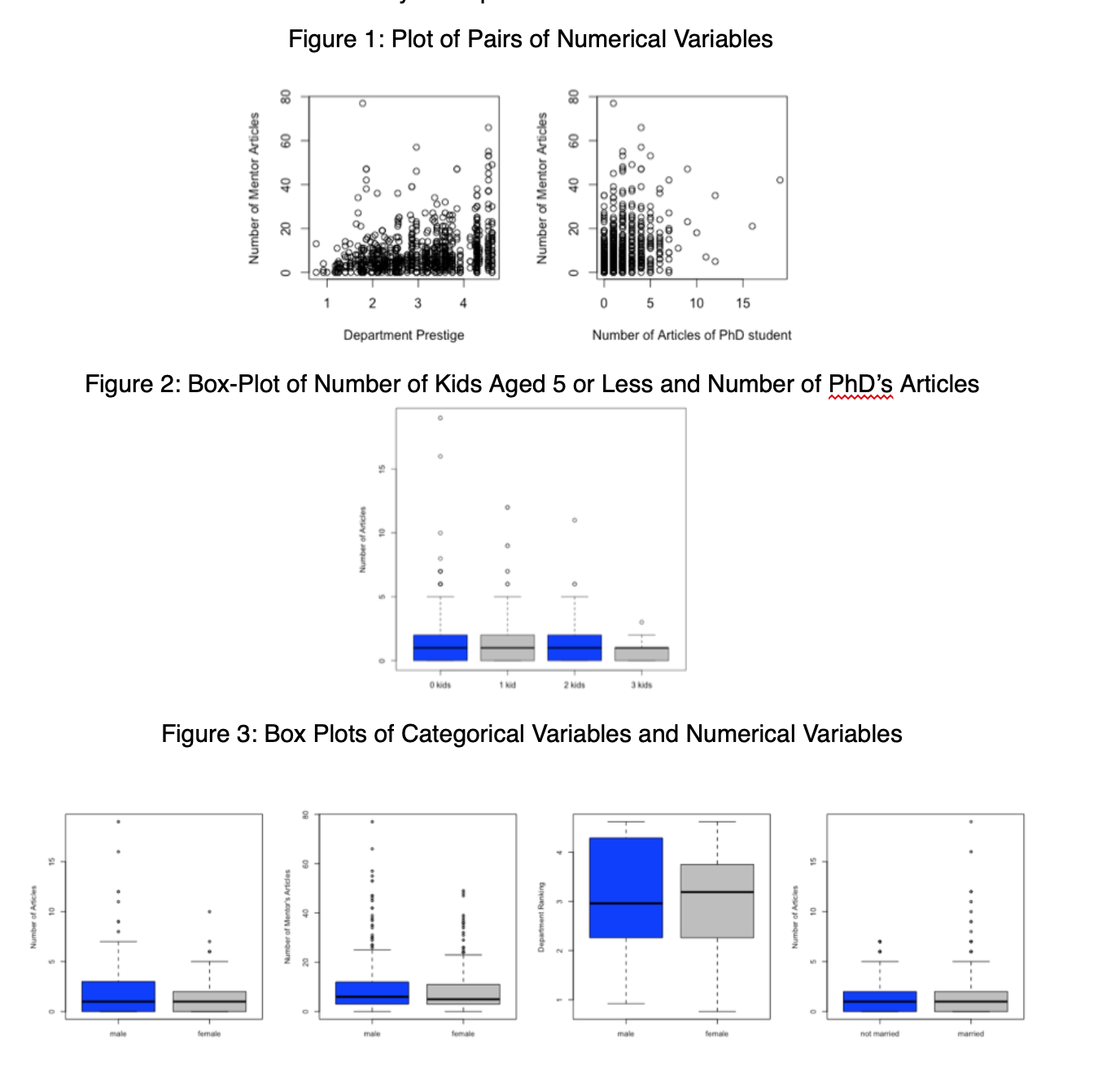
Graphical EDA Figure 1 shows the relationships between mentor and dept, art. It is hard to tell due to overplotting, but there appears to be a positive correlation between dept and mentor, with a correlation coefficient of 0.26. For both art and mentor, the main part of the distribution is similar in both genders (Figure 3), but the distribution has larger spread in males, and as a result the men who publish the most articles (or who have mentors who publish more) publish more than the women who publish the most. The distribution of the prestige of the department is similar amongst men and women, with men having a lower median but a larger upper quartile (Figure 3). Although the main distribution is similar, among married PhD students there are significantly more outliers with more published articles than expected (Figure 3). For students with 0, 1, or 2 children under 5, the main distributions are also similar, but students with fewer children have more high-publishing outliers (Figure 2). The distribution for students with 3 children has notably less spread and is more concentrated towards 0.

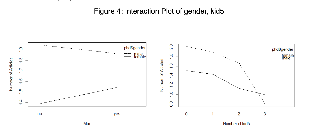
Another important aspect is checking for interactions between variables of interest. It is important, because including any significant interaction effect in our model may result in better understanding of the relationship of interest, leading to better predictions. We may notice (Figure 4) that there appears to be a significant interaction between the number of children and the gender, in particular male students have a large drop in productivity when they have three children, whereas female students experience a much less significant drop. However, only 16 students in the dataset have 3 children, and so it is not wise to draw any significant conclusions from this.

1. Model Selection Throughout the analysis, we will use Poisson log-linear model. Poisson regression is used to predict a dependent variable that consists of count data given one or more independent variables. We use Poisson regression, because our aim is to predict a dependent variable (art) which consists of count data and Poisson model is the most basic model which can do that. To be more precise, the Poisson regression model is Generalized Linear Regression model that assumes: The responses are non-negative integers that are independent of each other Each response follows the Poisson distribution with the mean λi and λi, P(yi = k|λi) = λki e−λi /k! θi =logλi =Xiβ, where X and B are matrices. Our dataset satisfies the following Poisson assumptions: The dependent variable, art, includes non negative integers and they have no natural upper bound, Our five hypothesized independent variables are either continuous or categorical (see Table 1 and Table2). Each observation is independent of the other observations. The distribution of dependent variable follow a Poisson distribution. In another word, the model predicts the observed counts well (see Figure 5). The variance has the same value as the mean (see Figure 6). Each variable has 915 valid observations and their distributions seem quite reasonable. The unconditional mean and variance of the dependent variable are not extremely different. We are making an assumption that, for each student, the independent variables, their mean productivity is equal to the variance of their productivity.

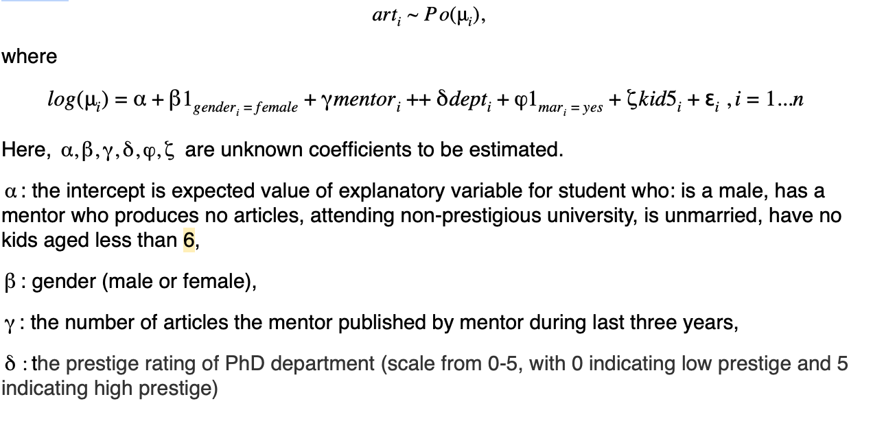
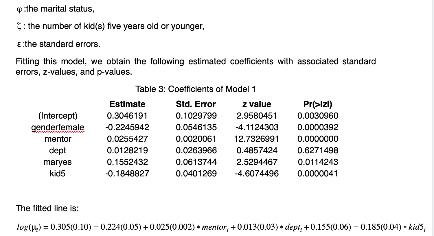
We decided to proceed to select model based on stepwise regression, to be more precise backward selection. We begin with simple poisson model including with all five covariates. We iteratively remove the least contributive predictor, and stops when we have a model where all predictors are statistically significant. As a result,we have chosen two models based on simplicity of interpretation and comparisons of fit. To see code to other models we tested please refer to Appendix 2. - let’s include other models we did in the Appendix 2 3.1 Model 1 In Model 1 we hypothesize that all covariates influence the dependent variable, and that there is no interaction between any of the covariates. This model seems reasonable, because all mentioned covariates might have impact on productivity of a biochemistry PhD students, and as noted in section 2.2 the interaction have no significant impact. Algebraically, this fits the model

Here the standard errors are in brackets. We include all five variables in the model 1, and variables gender=female and kid5 have negative effects on the articles’ productivity of a biochemistry PhD students, the others have positive effects. In addition, considering each coefficient, dept has a large p-value - around 0.63, meaning it may not be beneficial to include it in the model. We further inspect this issue using diagnostic plots.

The residuals do appear to be uncorrelated with the fitted values, and appear to to increase in variance as the fitted value increases - this is as we would expect, as in a Poisson model, mean is equal to variance (Figure 6).

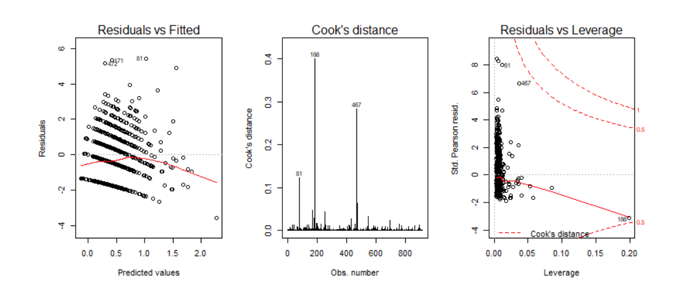
We may notice that there are three observations with high Cook’s distance - 81, 186, and 467. Table 4: Observations with high Cook’s distance

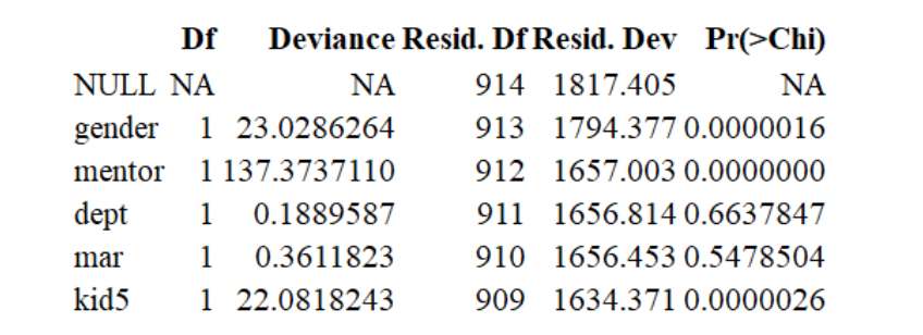
Observations 81 and 467 are the students who published the largest number of articles, 16 and 19, and observation 186 is a student who published only 1 article, but had a mentor who published 77, the largest value in the dataset. Observations 81 and 467 have unusual response values, but their low leverage means they are located in the interior of the dataset, so we shall leave them. Although a good practise is not removing any data which are correct, however in this case variable 186 has high leverage, around 0.2, meaning it is far from the other data points, and high cook’s distance, which distorts the fitted response values and might negatively impact the predictive ability of our model. Hence, we shall exclude it from further analysis, allowing us to focus on the model where the majority of the data points are. We now fit a simpler model, Model 2, dropping the dept term, and perform an analysis of variance(ANOVA) test to see if there drop in deviance from Model 2 to Model 1 is significant.

3.2 Model 2 Based on findings during analysis of model 1, we propose model 2. Model 2 includes four explanatory variables: kid5, mar, mentor, gend, with no interaction terms. Algebraically, we fit this model

Under the null hypothesis that the more complicated model, Model 1, is no better a fit than Model 2, we obtain a test statistic of .040, which, when referred to a 12 distribution, yields a p-value of 0.84, suggesting the drop in deviance in the more complicated model could just be down to chance. We thus do not reject the null hypothesis, and conclude there is insufficient evidence that Model 1 is a better fit than Model 2. Fitting the model 2, we obtain the following estimated coefficients with associated standard errors, z-values, and p-values.

Here the standard errors are in brackets. We now include only four independent variables, (except the dept), in model 2. And all of these coefficients become significant, so we stop here. We found the direction of the effects behave the same as mode 1. We may now proceed to the conclusion and interpretation.

1. Conclusion and interpretation

As a result of our investigation, the we choose Model 2 as our final model

As we can see, five variables such as gender female, mentor, marriage = yes and kid5 are included and only the variable gender female and kid 5 have negative effect for this log linear model. The response log(i) will increase when the rest of variables increase.

First of all, the Model 1 which is given as glm1 are investigated at the beginning of the model fitting part. By seeing from the diagnostic plots, we removed the observation 186(outlier) since it has high leverage, which means it is far from the other data points.

Considering each coefficient, the big p value for dept are observed from the R output, and meaning it may not be beneficial to include it in the model, therefore dropping the dept term, and it turns out our Model 2( without depth) is better fit than Model 1 under the null hypothesis.

We also consider the interaction effect, but it shows no better than Model 2 ,therefore we decide Model 2 is our final model which is already shown above.

Because the terms are additive in log(i), they are multiplicative in i. We can thus interpret the coefficients as follows. We would expect a male, unmarried PhD student with no children and a mentor who produces no articles to produce exp(0.317)1.37 We expect female PhD students to publish at about exp(−0.226)0.780 articles over their three years. For each article produced by their mentor, we expect a student to increase the number of articles they publish by a factor of exp(0.0282)1.029 the rate of an identical male counterpart, and married students to publish at exp(0.159)1.172 the rate of an identical unmarried counterpart. Finally, for each child under the age of 5 a student has, we expect their rate of publishing to be multiplied by a factor of exp(−0.185)0.831

After interpreting all the coefficients, we can make some predictions of productivity based on our final model within the range of every variables: Kid5 : [0,3] Mentor publications : [0,48]

For example, for a female married biochemistry PhD student, with no children under 5, who has a mentor who published 20 articles in the last three years, we would expect the number of articles they have published in the last three years to be Poisson distributed with mean exp(0.317−0.226+0.159+200.0282)=2.260.

Finally, we need to be aware of limitations of predicting power of our model. In the introduction we have assumed independence and external validity of our model. We assume that samples of Biochemistry PhD students were taken independently from different schools and different countries. This assumption allow us to use model to predict the productivity of any biochemistry PhD student. If any of the mention assumptions doesn’t hold, then predictions based on built model might lead to wrong conclusions.