Using CNN’s for Image classification

%matplotlib inline

import os
import numpy as np
import matplotlib.pyplot as plt
import cv2

import keras
from keras import metrics
from keras.preprocessing.image import ImageDataGenerator, array_to_img, img_to_array, load_img
from keras.models import Sequential
from keras.layers import Dense, Dropout, Activation, Flatten, BatchNormalization
from keras.layers import Conv2D, MaxPooling2D

img_width = 50
img_height = 50
num_classes = 2
DATA_DIR = './data/'
image_filenames = [i for i in (os.listdir(DATA_DIR))] # use this for full dataset

# Create test labels - "1" for cat, "0" for dog based on file name. When found, in general images are correctly assigned
# apart from some exceptions (eistein, wrong labels etc.). The number of mistakes is however not significant

labels=list()
for i in range(len(image_filenames)):
    if "cat" in image_filenames[i]:
        labels.extend(["cat"])
    elif "dog" in image_filenames[i]:
        labels.extend(["dog"])
    else:
        labels.extend("unknown")

# Create a data frame with image filename and rspective lable

import pandas as pd
image_filenames=pd.DataFrame(image_filenames)
image_filenames["labels"]=labels
image_filenames.columns=["dir", "labels"]
print(image_filenames)

# I divide dataset fot training, validation and testing sets

training_data= image_filenames[:][0:4799]                                                                                          
test_data = image_filenames[:][4800:5399]  
validation_data = image_filenames[:][5400:5999]

from PIL import Image # Library to access images

# print(Image.open(image_filenames[0][0])) # Images have different sizes
# print(Image.open(image_filenames[0][3000]))

Image.open("./data/"+image_filenames["dir"][3000]).show() # Display image to make sure everything above works

from keras_preprocessing.image import ImageDataGenerator

# Before I train the Neural Network, I need to prepare data. Convinent tools are generators. I set them up
# such that they standarise data, scale them to picture 50x50 pixels, set it up as a binary classification
# and take them from given directory

# I also include data agumentation in the form of such as zooming,  rotation, flipping,
# Image agumentation helps to make model more generisible and prevents overfitting

datagen = ImageDataGenerator(
    rescale=1./255,
    shear_range=0.1,
    zoom_range=0.1,
    horizontal_flip=True)

# I cal flow_from_dataframe to access training pictures by filenames, set fixed seed for reproductability, target
# size 50 as required and I shuffle the data

train_generator = datagen.flow_from_dataframe(
    dataframe=training_data,
    directory='/Users/adamgajtkowski/Desktop/Assignment/data/',
    x_col="dir",
    y_col="labels",
    target_size=(50,50),
    class_mode="binary",
    shuffle=True,
    seed=42)

# I cal flow_from_dataframe to access testing pictures by filenames, set fixed seed for reproductability, target
# size 50 as required and I don't shuffle the data to make sure that labels fit when I compute cofusion matrix later

test_generator= datagen.flow_from_dataframe(
    dataframe=test_data,
    directory='/Users/adamgajtkowski/Desktop/Assignment/data/',
    x_col="dir",
    y_col="labels",
    target_size=(50,50),
    class_mode="binary",
    shuffle = False,
    seed=42)


# I cal flow_from_dataframe to access validation pictures by filenames, set fixed seed for reproductability, target
# size 50 as required and I shuffle the data

validation_generator = datagen.flow_from_dataframe(
    dataframe=validation_data,
    directory='/Users/adamgajtkowski/Desktop/Assignment/data/',
    x_col="dir",
    y_col="labels",
    target_size=(50,50),
    class_mode="binary",
    seed=42,
    shuffle=True)

# Setting simple Neural Network, consisting of one convolutional layer, activation functions relu (final sigmoid)
# one max-pooling layer and two dense layers. I set 'adam' optimizer, which is gradient descent with adapive weights
# In the last line I fit the generator, and set validaiton data defined above. I set 17 epochs and 100 steps per
# epoch, as this increase the learning rate

convnet = Sequential()
convnet.add(Conv2D(32, (3,3), input_shape=(50, 50,3), data_format="channels_last"))
convnet.add(Activation('relu'))

convnet.add(MaxPooling2D(pool_size=(2, 2)))
convnet.add(Flatten())  # this converts 3D to 1D vectors

convnet.add(Dense(32))
convnet.add(Dense(1))

convnet.add(Activation('sigmoid'))

convnet.compile(loss='binary_crossentropy',
              optimizer='adam',
              metrics=['accuracy'])

model_con=convnet.fit_generator(
        train_generator,
        steps_per_epoch=100,
        epochs=17,
        validation_data=validation_generator,
        validation_steps=20)

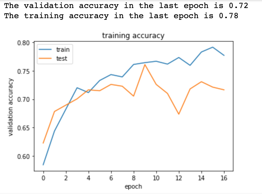
# The accuracy of this simple network is relatively low. Given it's binary problem, I would expect the validation accuracy
# to be above 90. This simple network results in validaiton accuracy of around 70. The training accuracy
# is a bit higher (77%). This sugests that overfitting is not a big problem in case of this model (as it doesn't learn the data).
# Overall, not the highest accuracy might be a consequence of low amount of pictures in training set
# as neural networks usually need high amount of data to perform classification well.

# print(model_con.history.keys()) # names available
print('The validation accuracy in the last epoch is', round(model_con.history['val_acc'][16],2)) # print valuation accuracy - most recent is 72%, which is not the highest in the binary setting
print('The training accuracy in the last epoch is',round(model_con.history['acc'][16],2)) # print training accuracy

# Plotting required training accuracy and validation accuracy, (adding respective titles and legend)
plt.plot(model_con.history['acc'])
plt.plot(model_con.history['val_acc'])
plt.title('training accuracy')
plt.ylabel('validation accuracy')
plt.xlabel('epoch')
plt.legend(['train', 'test'], loc='upper left')
plt.show()

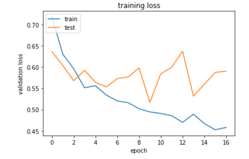
# Plotting required training loss and validation loss, (adding respective titles and legend)
plt.plot(model_con.history['loss'])
plt.plot(model_con.history['val_loss'])
plt.title('training loss')
plt.ylabel('validation loss')
plt.xlabel('epoch')
plt.legend(['train', 'test'], loc='upper left')
plt.show()

# getting accuracy of predictions base on test data
predictions_accuracy=convnet.evaluate_generator(test_generator, steps=19)[1]
print('Accuracy of predicitons is:',round(predictions_accuracy,2))

# I cal predict_generator to predict probabilities that given picture is classified to either 'cat', or 'dog'
# First I need to reset the test generator, to make sure testing data are in the right order
test_generator.reset()
pred1=convnet.predict_generator(test_generator,steps=19)

from sklearn.metrics import precision_recall_curve, confusion_matrix

# Predicting pictures based on probability (because its output ranges between 0 and 1)
# label '0' means cat, label '1' means dog

predict1=list()
for x in pred1:
    if x>0.5:
        predict1.extend("1")
    elif x<=0.5:
        predict1.extend("0")

predict1 = list(map(int, predict1))  # set preddictions as a list of ints

print(metrics.binary_accuracy(test_generator.classes,predict1))  # print predictions
print('Confusion Matrix')
print(confusion_matrix(test_generator.classes, predict1)) # Consufion matrix

fig = plt.figure(figsize=(10,5))

# Setting a title for the set of plots
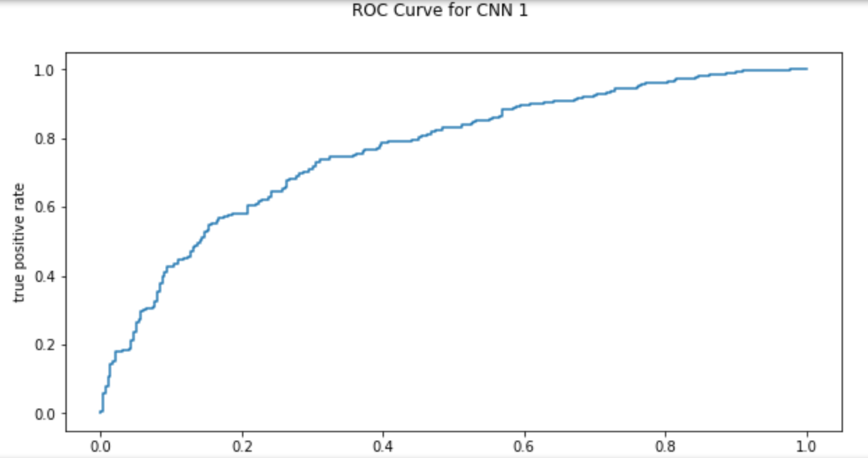
fig.suptitle('ROC Curve for CNN 1')

# Plotting the ROC curve
from sklearn.metrics import roc_curve
fpr, tpr, thresholds = roc_curve(test_generator.classes, pred1, pos_label=1)
ax1 = plt.subplot(1, 1, 1)
ax1.set_xlabel('false positive rate') # axis titles
ax1.set_ylabel('true positive rate') # axis titles
ax1.plot(fpr, tpr) # plotting

from sklearn.utils.fixes import signature
from sklearn.metrics import precision_recall_curve

#plotting precision-recall curve
precision, recall, _ = precision_recall_curve(test_generator.classes, pred1, pos_label=1)
fig = plt.figure(figsize=(5,5))
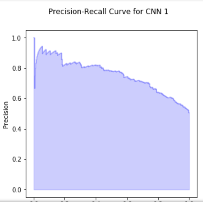
fig.suptitle('Precision-Recall Curve for CNN 1')

step_kwargs = ({'step': 'post'}
               if 'step' in signature(plt.fill_between).parameters
               else {})

plt0 = plt.subplot(1, 1, 1)
plt0.step(recall, precision, color='b', alpha=0.2,
         where='post')
plt0.fill_between(recall, precision, alpha=0.2, color='b', **step_kwargs)

plt0.set_xlabel('Recall')
plt0.set_ylabel('Precision')

# While the training accuracy increases with epochs (meaning model learns the data)
# the validation accuracy plateau around level 0.7 after 4 epochs
# This result is fairly poor and suggests that model should include more pictures, or
# higher quiality pictures (ex. higher resolution).
# Although the prediction accuracy based on test data is 0.70
# The ROC curve is far from upper left corner, precision recall curve is quire far away from upper right corner
#  and confusion matrix show that there is significant amount of true negatives and false positives
# Overall, the model is not bad given small training dataset but
# I would suggest using more data for training, as well as using more complex model (more layers)

from keras.callbacks import ModelCheckpoint

# I add to safe model with best weights - will use that in the last exercise in order to display the saliency map
checkpointer = ModelCheckpoint(filepath="best_weights.hdf5",
                               monitor = 'val_acc',
                               verbose=1,
                               save_best_only=True)

# Specifying more complex model, including three convolutional layers with relu activation function, three max pooliing
# layers, later I flatten features to 1D. In this case, I also use dropout once to increase the generasibility
# Fitting the model remains the same as above (apart from callbacks to safe best weight)
model = Sequential()

model.add(Conv2D(32, (3,3), input_shape=(50, 50,3), data_format="channels_last"))
model.add(Activation('relu'))
model.add(MaxPooling2D(pool_size=(2, 2)))

model.add(Conv2D(64, (3,3)))
model.add(Activation('relu'))
model.add(MaxPooling2D(pool_size=(2, 2)))

model.add(Conv2D(64, (3,3)))
model.add(Activation('relu'))
model.add(MaxPooling2D(pool_size=(2, 2)))

model.add(Flatten())  # flatten features to 1D
model.add(Dense(128))
model.add(Activation('relu'))
model.add(Dropout(0.5))
model.add(Dense(1))

model.add(Activation('sigmoid'))

model.compile(loss='binary_crossentropy',
              optimizer='adam',
              metrics=['accuracy'])

model_2=model.fit_generator(
        train_generator,
        steps_per_epoch=100,
        callbacks=[checkpointer],
        epochs=17,
        validation_data=validation_generator,
        validation_steps=20)

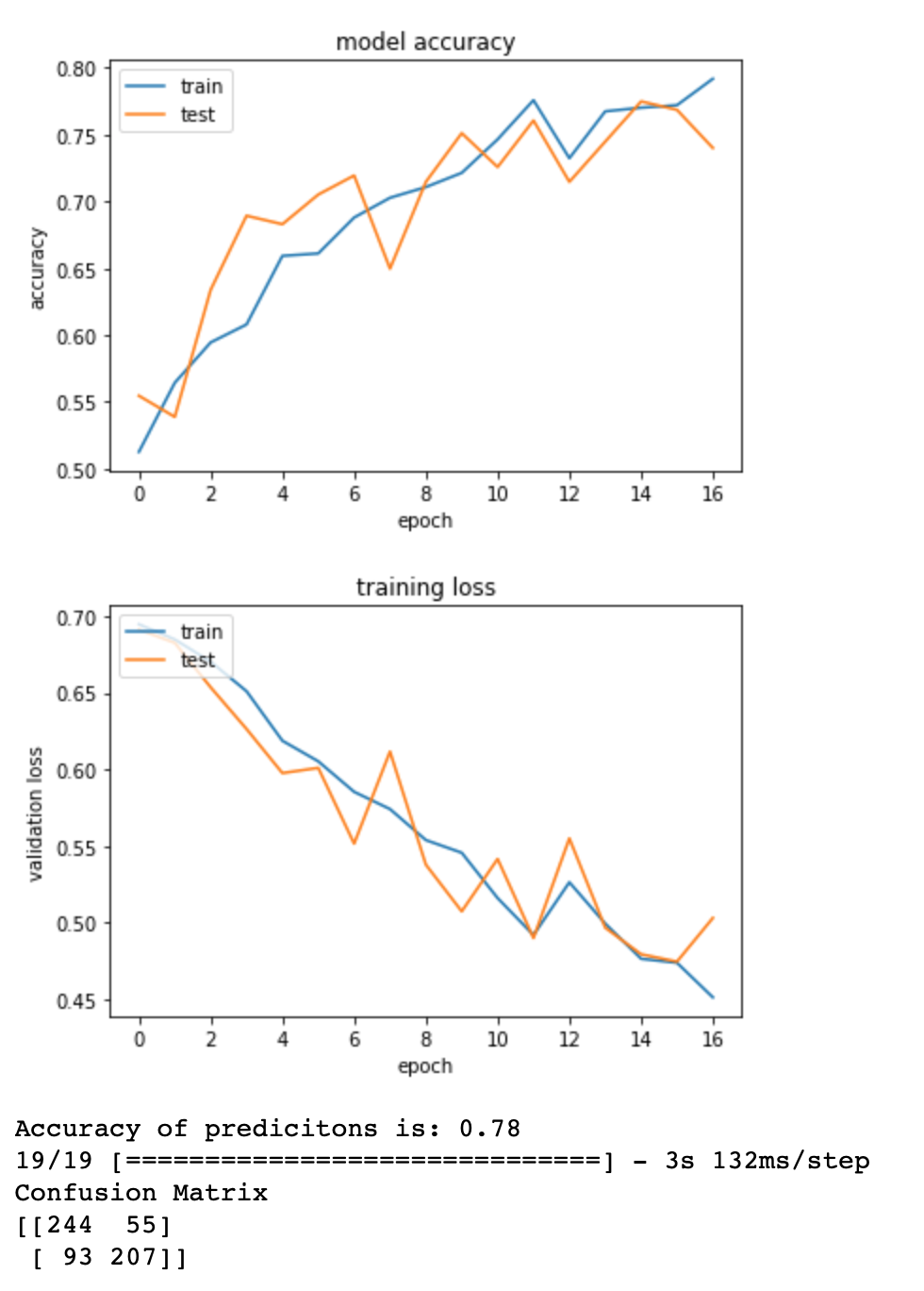
# The higest valuation accuracy in case of this model is 79, compared to previous more simple model where
# the validation accuracy was just around 70, it is a significant imporvement. The training accuracy increases
# as validation accuracy increases, at a similar pace suggesting that we don't have a problem with overfitting.
# Overall, the validation accuracy increased by almost 10%, suggesting that adding mulitple convolutional
# layers and dropout is benefitial to our model.

# I have attempted to tune parameters by changing activation function, amount of conv layers (4,6),
# changing optimizer, adding more dropout layers, increaseing/decreasign epochs however the proposed
# model performed best and results in accuracy of predictions 78%

# Output the validation accuracy and training accuracy
print('The validaiton accuracy in the last epoch is', round(model_2.history['val_acc'][16],2)) # print valuation accuracy - most recent is 75%, which is not the highest in the binary setting
print('The training accuracy in the last epoch is',round(model_2.history['acc'][16],2)) # print training accuracy

# Plot the training accuracy and validaiton accuracy
plt.plot(model_2.history['acc'])
plt.plot(model_2.history['val_acc'])
plt.title('model accuracy')
plt.ylabel('accuracy')
plt.xlabel('epoch')
plt.legend(['train', 'test'], loc='upper left')
plt.show()

# Plotting required training loss and validation loss, (adding respective titles and legend)
plt.plot(model_2.history['loss'])
plt.plot(model_2.history['val_loss'])
plt.title('training loss')
plt.ylabel('validation loss')
plt.xlabel('epoch')
plt.legend(['train', 'test'], loc='upper left')
plt.show()


# Predict the testing data based on trained network
predictions_accuracy=model.evaluate_generator(test_generator, steps=5)[1]

# Output the accuracy of predictions
print('Accuracy of predicitons is:',round(predictions_accuracy,2))

# I cal predict_generator to predict probabilities that given picture is classified to either 'cat', or 'dog'
# First I need to reset the test generator, to make sure testing data are in the right order
test_generator.reset()
predictions_2=model.predict_generator(test_generator,verbose=1, steps= 19)

# Predicting pictures based on probability (because its output ranges between 0 and 1)
# label '0' means cat, label '1' means dog
pred2=list()
for x in predictions_2:
    if x>0.5:
        pred2.extend("1")
    elif x<=0.5:
        pred2.extend("0")

pred2 = list(map(int, pred2)) # set preddictions as a list of ints
predictions_2=list(map(float, predictions_2)) # Map probabilities to floats

# Print accuracy based on training data and confusion matrix
print('Confusion Matrix')
print(confusion_matrix(test_generator.classes, pred2))

fig = plt.figure(figsize=(10,5))

#  Print ROC curve, setting a title for the set of plots
fig.suptitle('ROC Curve for CNN 1')

from sklearn.metrics import roc_curve
fpr, tpr, thresholds = roc_curve(test_generator.classes, predictions_2, pos_label=1)
ax1 = plt.subplot(1, 1, 1)
ax1.set_xlabel('false positive rate') # axis titles
ax1.set_ylabel('true positive rate') # axis titles
ax1.plot(fpr, tpr) # plotting

# Now plot the precision recall curve, with respective labels
precision, recall, _ = precision_recall_curve(test_generator.classes, predictions_2, pos_label=1)

fig = plt.figure(figsize=(5,5))
fig.suptitle('Precision-Recall Curve for CNN 2')

step_kwargs = ({'step': 'post'}
               if 'step' in signature(plt.fill_between).parameters
               else {})

# Plotting recall curve for Decision Tree
plt0 = plt.subplot(1, 1, 1)
plt0.step(recall, precision, color='b', alpha=0.2,
         where='post')
plt0.fill_between(recall, precision, alpha=0.2, color='b', **step_kwargs)

plt0.set_xlabel('Recall')
plt0.set_ylabel('Precision')

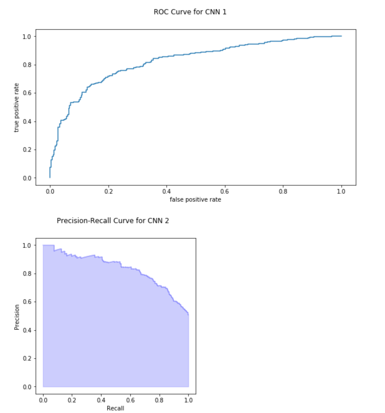
# The testing and training accuracy are higher compared to the simple CNN. The test and
# validation accuracy are converging over time together (means no overfitting), the accuracy of predictions
# based on this network is higher just by 8% points (increase from 70 to 78).
# Again, the possible reason for this low performance is not enough training data.

# The confusion matrix, ROC curve and Precision-Recall graphs are improved compared to above model.
# Although the difference is mariginal, this model proves that more complex neural network,
# with more convolutional and training layers is benefitial for testing accuracy. The drawback of this
# complex layer is higher training time.

# The code comes from: https://towardsdatascience.com/visualizing-intermediate-activation-in-convolutional-neural-networks-with-keras-260b36d60d0
# I was unable to do it using the above link
import glob
import matplotlib
from matplotlib import pyplot as plt
import matplotlib.image as mpimg
import numpy as np
import imageio as im
from keras import models
from keras.preprocessing import image
from keras.preprocessing.image import ImageDataGenerator

# specifying path for the image on which we will visualise the layers
img_path = './data/dog.1.jpg'

# I load the image, normalise and transform to required size
img = image.load_img(img_path, target_size=(50, 50))
img_tensor = image.img_to_array(img)
img_tensor = np.expand_dims(img_tensor, axis=0)
img_tensor /= 255.
img.show() # Displays the image of a dog

# Load best weights specified by latest model
model.load_weights('best_weights.hdf5')

# Define outputs for all layers
layer_outputs = [layer.output for layer in model.layers]

# Creates a model that will return these outputs, given the model input
activation_model = models.Model(inputs=model.input, outputs=layer_outputs)

# Load the above image of the dog to pass it to layers
activations = activation_model.predict(img_tensor)

# array including list of the layers
layer_names = []
for layer in model.layers[:8]:
    layer_names.append(layer.name)
# Specify the number of images per row
images_per_row = 16

# This code and comments comes from above link and display the  fetures map
for layer_name, layer_activation in zip(layer_names, activations):
    n_features = layer_activation.shape[-1] # Number of features in the feature map
    size = layer_activation.shape[1] #The feature map has shape (1, size, size, n_features).
    n_cols = n_features // images_per_row # Tiles the activation channels in this matrix
    display_grid = np.zeros((size * n_cols, images_per_row * size))
    for col in range(n_cols): # Tiles each filter into a big horizontal grid
        for row in range(images_per_row):
            channel_image = layer_activation[0,
                                             :, :,
                                             col * images_per_row + row]
            channel_image -= channel_image.mean() # Post-processes the feature to make it visually palatable
            channel_image /= channel_image.std()
            channel_image *= 64
            channel_image += 128
            channel_image = np.clip(channel_image, 0, 255).astype('uint8')
            display_grid[col * size : (col + 1) * size, # Displays the grid
                         row * size : (row + 1) * size] = channel_image
    scale = 1. / size
    plt.figure(figsize=(scale * display_grid.shape[1],
                        scale * display_grid.shape[0]))
    plt.title(layer_name)
    plt.grid(False)
    plt.imshow(display_grid, aspect='auto', cmap='viridis')

    # It seems that the conv2d_2 layer is very useful for the shape recognition, while
    # later conv2d are not that useful to differentiate between pictures (at least as for human eye).
    # This confirms above findings, that more complex neural netword does not neccessarly
    # performs significantly better, as the accuracy of test data
    # increased by just 5% points. The drawback of more complex network is that it takes significantly more
    # time to train it. Thus I would reccomend to use simple CNN in case these is lots of data,
    # or in our case it actually make sense to use more complex network, as the training time is not
    # much higher, but the results are better.