Data Cleaning and Model Selection
This report investigates the relationship between weight of plastic conkers and their dimensions. The dataset we analyse includes 129 observations recording three variables each: the weight (in grams) the maximum dimension (in millimetres) and the minimum dimension (in millimetres).
Before we begin to analyse it, is important to be aware of the limitations of this dataset. Firstly, we analyse a relatively small sample. That might result in biased estimators. Biased estimators mean that the parameters estimated from a sample are not truly representative to the population. We also have no information about the data generating process (DGP). That means that we do not know:
• How the data was collected,
• If the instruments used to collect the measurements were calibrated,
• If the plastic conkers were randomly selected or did they come from the same batch.
As this report aims to investigate the relationship between all plastic conkers and their dimensions, we need to assume that the data records are not distorted by any of the above issues.
2.0 Exploratory Data Analysis
Before we analyse the data, we run through the data set to look for non-integer type values, or values that are not within reasonable range. After running through the data we remove the observation with index 129 as it records weight of the conker to be 0 grams which is not possible. This could be due to a mistake when recording the data. We assume that this observation is not informative to make further inference about characteristics of the population.
We also run through the data to check that there is the same number of entries for all 3 variables. We check if the maximum length recorded is bigger than the corresponding minimum length. We do not find any further inconsistencies.
With the removal of observation indexed 129, the analysis carried out below is based on the remaining 128 observations.
2.1 Numerical Exploratory Data Analysis
The mean and medians of all variables are close to each other (Table 1). This suggests that the variables might be symmetrically distributed. We can also notice that variable minimum length has higher standard deviation than maximum length. This suggests that the range of values for minimum length are quite spread out from the mean.
We will now look at the skewness and the kurtosis for each variable (Table 2). Skewness is a measure of lack of symmetry. Kurtosis is a measure of whether the data are heavy tailed or light tailed relative to a normal distribution. Data set with high kurtosis value tends to have outliers while data set with low kurtosis value tends to lack outliers. The kurtosis value of a Gaussian distribution is 3 (also included in the table).
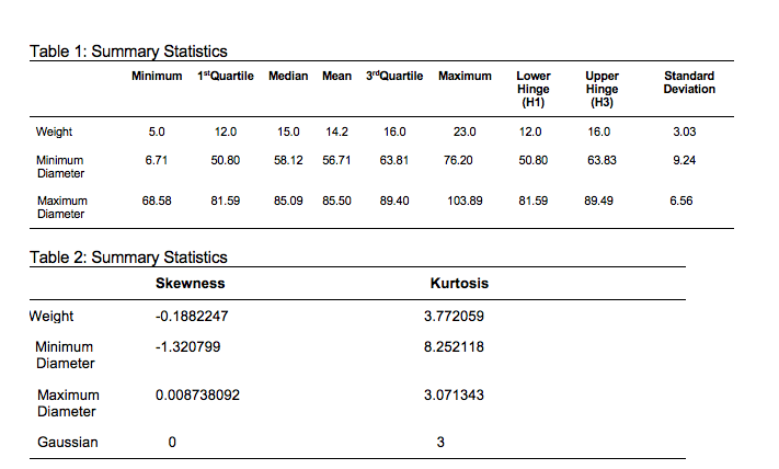
From the table we can see that both weight and minimum diameter have negative skewness, indicating that the distribution is skewed to the left. Maximum diameter has skewness relatively close to zero, indicating that the distrib›ution could be symmetrical.
Both weight and maximum diameter have kurtosis value close to that of a Gaussian distribution. High kurtosis of minimum diameter indicates that there might be an outlier.
These values only give us a general idea of the distribution as the sample size is small.
2.2 Graphical Exploratory Data Analysis
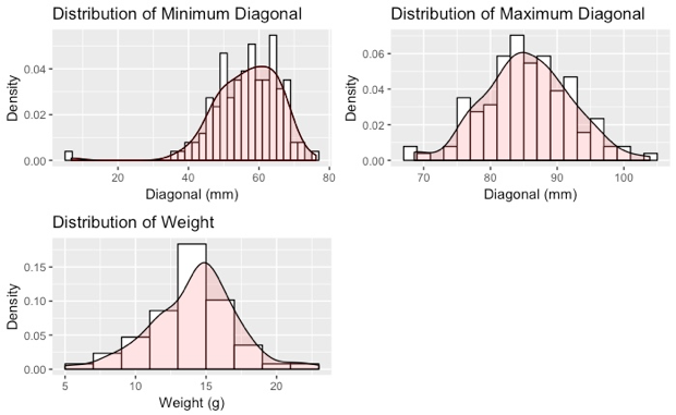
Figure 1 shows the distribution (using histogram and density function) of variables minimum diameter, maximum diameter and weight of plastic conker respectively. The histograms suggest that both the minimum and maximum diameter has outliers on the left side of the distribution. As the outlier for minimum diameter is quite far from the rest of the data, this might have contributed to the relatively big kurtosis value and negative skewness. Weight and Maximum variables appear to have similar distribution, where points are symmetrically distributed around one value. From the histogram we can also say that the variables minimum diameter and weight are skewed to the left.
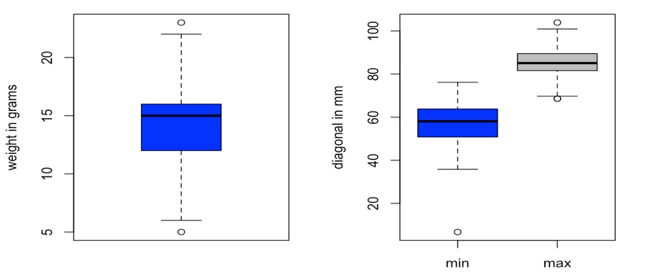
Figure 2 shows the box-plots for variables weight, maximum diameter, and minimum diameter respectively. Box plot includes 5 elements: high outliers, max, upper-hinge, median, lower-hinge, min, low outliers. We may notice that the minimum diameter has much higher spread than the maximum diameter, as suggested by the higher standard deviation in the summary statistics above. In addition, the outlier for the minimum diameter is further from the lower hinge as compared to the outliers of weight and maximum diameter.
The median of weight is nearer to the upper hinge than the lower hinge, suggesting that the distribution for weight is skewed to the left. Outliers of weight and max diameter lie close to its maximum/minimum.
2.3 Outliers
Graphical EDA suggests existence of outliers in case of all variables of the dataset. The analysis below intends to identify all outliers and check if they have significant impact on the distribution of a given variable. If they do, it may lead to wrong conclusions about the relationship between the conker’s weight and its dimensions. We use following formulas to identify outliers:
, where is the lower hinge —–(1) where is the upper hinge —–(2) IQR = 3rd quartile – 1st quartile
We decided to use hinges to be consistent with outliers identified by estimates from box-plots.
The outliers for the following variables are Weight (in grams): 5, 23 Maximum Diameter (in mm): 68.58, 68.63, 69.75, 103.89 Minimum Diameter (in mm): 6.71
For both weight and maximum diameter, the mean, variance, skewness and kurtosis do not change significantly with the removal of the outliers (Table 3).
With the removal of the outlier, the variance of the minimum diameter decreases significantly. The distribution is skewed less to the left with kurtosis value closer to that of the Gaussian distribution. We will not remove this data point but will take note of it when building the model and check if its removal changes results significantly.
In general it is a good practise to not remove an observation just because it is an outlier. An outlier can still possess some important information about possible extreme values within a given distribution of a variable. In addition we do not know if the outlier is due to an error in measurement or mistake in recording, thus we do not remove› it.

3.0 Model Selection
We have decided to use a linear model in the form to explain the relationship between plastic conkers and their dimensions. We are considering the following model, where we set variable weight ( ) as the response variable, minimum diagonal ( ) and maximum diagonal ( ), as the explanatory variables. We denote random error as . We build this model because we believe that both maximum diagonal and minimum diagonal are related to the weight of a plastic conker. The regression model intends to discover how the weight of plastic conkers changes with the change in minimum/maximum diagonal.
We use method of least squares to find an estimate for the parameters, , and . Below are some assumptions made on the response variables
- They are normally distributed
- They are independent
- They have constant variance (homoscedasticity)
- The mean structure of the is a linear function of the parameters. We will check through these assumptions with suitable plots at the end of this section.
When we plot variables against each other (Figure 3), it seems that there is a linear relationship between them. That is why we will start with the linear model that includes both the maximum and minimum diameter as the explanatory variables. Below we consider 2 models which best fit our data.

3.1 Model 1 The F-values for the minimum diameter and maximum diameter are 104.4 and 111.1 respectively. Both values exceeded F(1, 125, 0.95) = 3.916932 indicating a statistically significant contribution by both variables. This means that we have strong evidence to reject the null hypothesis that the coefficients are zero, in favour of an alternative hypothesis that they are different to zero.
It is worth noticing that models 1-2 all consist the same number of independent variables. That is why, to compare models in terms of how well they perform, we will use R^2 .
Multiple R^2 value of Model 1 is 0.6329. This means that the model explains approximately 63.2% of the variation in the dependent variable. We will come back to this number measure once we test other models.
If we look at the Cook’s distance (Figure 4) for this model, observation indexed 105 seems to be an influential point, whose removal leads to a large change in the analysis. From Section 2 we see that the removal of observation indexed 105 changes the variance of the minimum diameter significantly. Also, we may notice that observation indexed 105 shows really unusual dimensions for a plastic conker.We will now remove this point and carry out linear regression using model 1 again. We shall name the model without the influential point model 1B.
3.2 Model 1B From the ANOVA table, the F-values for both the minimum diameter and maximum diameter are large, indicating that both variables are statistically significant. It means that we again reject the null hypothesis that coefficients are 0 in favour of alternative hypothesis that coefficients are different to 0. Multiple of this model is 0.7212, stating that the model explains approximately 72% of the variation. We compare the multiple R^2value for both model 1 and model 1B.
The removal of observation indexed 105 leads to a significant increase in . For the model 2, we will only present the summary of the models with the removal of observation indexed 105, as we identified this point as an influential point. Please refer to the appendix for the summary of the of the model with the inclusion of observation indexed 105.
3.3 Model 2 - Without Influential Point
We decided to choose, as our second model, the one with log values as explanatory variables. Log transformation is a linear transformation which can smooth our data. In Section 2 we have found that some variables are skewed. We believe that taking log transformation can “normalize” our data and make it more symmetric. Another aspect of log transformation is the ease of interpretation. We have taken the log of explanatory variables. Then 1% increase in X_i will lead to change in .
We have found that all estimates are highly significant, thus we reject the null hypothesis in favour of alternative that coefficients are different to 0.
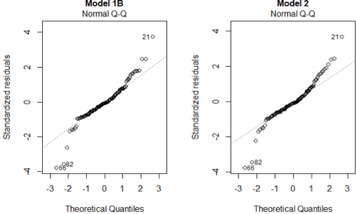
We shall now check the assumptions made at the start of the Section. 1) are normally distributed with the Q-Q plots
From the QQ plots, most of the points lie on the straight line for both models, suggesting that the assumption holds for both models. But the points in Model 1B seem to cluster more tightly around the straight line compared to Model 2.
2) The are independent 3) The mean structure of the is a linear function of the parameters.
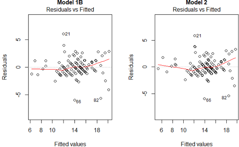
Both plots do not display any relationship between the fitted values and the residuals. We can infer that both assumptions hold for the models.
4) The have constant variance (homoscedasticity)
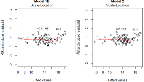
Based on scale-location plot, we do not find any trend in the variations for both models. Thus we can conclude that the assumption holds for both models.
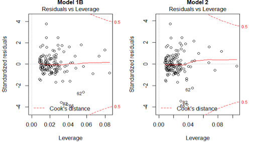
The residuals vs leverage plot helps us to identify influential point that might affect our linear regression model. Since there are no observations in the upper right and lower right corner, it suggests that there are no influential points for both models. In conclusion, the 4 assumptions hold for both Model 1B and Model 2.
4.0 Comparing the models and conclusion
Model 2 has a slightly higher R^2value suggesting that more variation is explained by Model 2 compared to the other. Furthermore, the sum of squares of residuals is also slightly lower suggesting that the square of the distance between the predicted values and the observed values is smaller. Because model 2 does not give a significant increase in both measurements and since the 4 assumptions hold for both models, which we saw from the diagnostic plots, the transformation is unnecessary. Thus we would choose the Model 1B to explain the relationship between the weight and the dimension of the conkers.
Model 1B states that when the minimum diameter increases by 1 mm, the weight will increase by 0.17g, similarly if the maximum diameter increases by 1mm, weight will increase by 0.27g. It is good to note that the equation can only be used to predict the weight for values of minimum diameter in the range [35.81,76.20] and maximum diameter in the range [68.58,103.89]. Otherwise we would need to extrapolate, however extrapolation might give a bad prediction.
It will be good to note that though the R^2value is high for this model, it does not imply that this model provides the best fit to the data set. It only implies that this model explains around 70% of the variation. Other models that better explain the relationship between weight and the dimensions may exist, possibly with more explanatory variables.
1.Data Cleaning
nut<-Nuts
weight<-nut$weight
max.length<-nut$max
min.length<-nut$min
size<-length(weight)
size2<-length(max.length)
size3<-length(min.length)
#We will first check that the size of the data is the same for all 3 variables.
all.equal(size2,size3)
## [1] TRUE
all.equal(size,size2)
## [1] TRUE
#We will first look for the wrong data type, for example non-integer and non positive value for weight

reasonable.weight<-function(){
 for(i in 1:size){
   if(is.numeric(weight[i])==FALSE){
     coordinate.type<-paste("Wrong type for coordinates:",i)
     print(coordinate.type)
   }
   if(weight[i]<=0){
     coordinate.range<-paste("Check range for coordinate",i)
     print(coordinate.range)
   }
 }
}
 reasonable.weight()
## [1] "Check range for coordinate 129"
#Data 129 will be removed since weight cannot be 0. We will now look for non integer value or non positive value for maximum length
reasonable.max.length<-function(){
 for(i in 1:size2){
   if(is.numeric(max.length[i])==FALSE){
     coordinate.type<-paste("Wrong type for coordinate:", i)
     print(coordinate.type)
   }
   if(max.length[i]<=0){
     coordinate.range<-paste("Check range for coordinate",i)
print(coordinate.range)
}
 }
}
reasonable.max.length()


#We will now look for non integer value or non positive value for maximum length
reasonable.min.length<-function(){
 for(i in 1:size3){
   if(is.numeric(min.length[i])==FALSE){
     coordinate.type<-paste("Wrong type for coordinate:", i)
     print(coordinate.type)
   }
   if (min.length[i]<=0){
     coordinate.range<-paste("Check range for",i)
print(coordinate.range)
   }
 }
}
reasonable.min.length()
reasonable.difference<-function(){
 for(i in 1:size2){
    if((max.length[i]-min.length[i]<=0)==TRUE){
     coordinate.range<-paste("Wrong value for row:",i)
     print(coordinate.range)
    }
 }
}


#We will now remove row 129 from the data set as weight is equal to 0.
nut<-nut[-129,]
weight<-nut$weight
max.length<-nut$max
min.length<-nut$min
size<-size-1
2.1 EDA Numerical
#Firstly we perform numerical EDA
summary(weight)
##    Min. 1st Qu.  Median Mean 3rd Qu.    Max.
##    5.0 12.0    15.0 14.2 16.0    23.0
summary(min.length)
##    Min. 1st Qu.  Median Mean 3rd Qu.    Max.
##   6.71  50.80 58.12  56.72 63.81 76.20
summary(max.length)
##    Min. 1st Qu.  Median Mean 3rd Qu.    Max.
##  68.58   81.61 85.09  85.50 89.40 103.89
fivenum(weight) #minimum, lower-hinge, median, upper-hinge, maximum
## [1]  5 12 15 16 23
fivenum(min.length)
## [1]  6.710 50.800 58.115 63.830 76.200
fivenum(max.length)
## [1]  68.580 81.585  85.090 89.485 103.890
sd(weight)
sd(min.length)
sd(max.length)
library(moments)
skewness(weight)# small skewed to the left
## [1] -0.1882247
kurtosis(weight) # weakly leptokurtic
## [1] 3.772059
skewness(min.length) # skewed to the left
## [1] -1.320799
kurtosis(min.length) # strongly leptokurtic
## [1] 8.252118
skewness(max.length) #almost no skewness
## [1] 0.008738092
kurtosis(max.length) # mesokurtic (in approximation)
## [1] 3.071343
2.2 EDA Graphical
par(mfrow=c(2,2))
library(gridExtra)
library(grid)
library(ggplot2)
library(lattice)
#R code for Figure 1:
grid.arrange(

(ggplot(as.data.frame(min.length), aes(x=min.length)) +geom_histogram(binwidth=2, aes(y=..density..),colour="black", fill="white")+geom_density(col=2) +geom_density(alpha=.2, fill="#FF6666")+labs(title="Distribution of Minimum Diagonal", x="Weight",y="Density")),

(ggplot(as.data.frame(max.length), aes(x=max.length)) +geom_histogram(binwidth=2, aes(y=..density..),colour="black", fill="white")+geom_density(alpha=.2, fill="#FF6666")+labs(title="Distribution of Maximum Diagonal",x="Diagonal", y="Density")),

(ggplot(as.data.frame(weight), aes(x=weight)) +geom_histogram(binwidth=2, aes(y=..density..),colour="black", fill="white")+geom_density(alpha=.2, fill="#FF6666")+labs(title="Distribution of Weight", x="Weight",y="Density")), nrow=2

)

par(mfrow=c(1,2))
#R code for Figure 2 :
boxplot(weight,col="blue", names=c("weight"),ylab="weight grams")
boxplot(min.length, max.length, col=c("blue","grey"),names=c("min","max"), ylab="diagonal in mm")
2.3 Outliers
# Identifying outliers for weight
for(i in weight){
 if(i>(16+1.5*4)){
   print(i)
 }
 if(i<(12-1.5*4)){
   print(i)
 }
}
## [1] 23
## [1] 5
# Identifying outliers for min
for(i in min.length){
 if(i>(63.81+1.5*13.01)){
   print(i)
 }
 if(i<(50.80-1.5*13.01)){
   print(i)
 }
}
## [1] 6.71
for(i in max.length){
 if(i>(89.40+1.5*7.79)){
   print(i)
 }
 if(i<(81.61-1.5*7.79)){
   print(i)
 }
}
## [1] 103.89
## [1] 68.63
## [1] 68.58
## [1] 69.75
3.(123) Modelling the relationship
pairs(nut) # Figure 3
lm1<-lm(weight~max.length+min.length,data=nut)# Model 1
lm1
##
## Call:
## lm(formula = weight ~ max.length + min.length, data = nut)
##
## Coefficients:
## (Intercept)   max.lengthmin.length
##    -16.2624       0.2791 0.1164
summary(lm1)
##
## Call:
## lm(formula = weight ~ max.length + min.length, data = nut)
##
## Residuals:
##     Min  1Q Median      3Q Max
## -5.4363 -0.8649 -0.1847  0.7681 8.8315
##
## Coefficients:
##              Estimate Std. Error t value Pr(>|t|)
## (Intercept) -16.26239    2.16914 -7.497 1.05e-11 ***
## max.length    0.27910 0.02648  10.540 < 2e-16 ***
## min.length    0.11638 0.01879   6.193 7.83e-09 ***
## ---
## Signif. codes:  0 '***' 0.001 '**' 0.01 '*' 0.05 '.' 0.1 ' ' 1
##
## Residual standard error: 1.848 on 125 degrees of freedom
## Multiple R-squared:  0.6329, Adjusted R-squared:  0.627
## F-statistic: 107.7 on 2 and 125 DF,  p-value: < 2.2e-16
anova(lm1)
## Analysis of Variance Table
##
## Response: weight
##             Df Sum Sq Mean Sq F value    Pr(>F)
## max.length   1 379.37 379.37   111.1 < 2.2e-16 ***
## min.length   1 356.50 356.50  104.4 < 2.2e-16 ***
## Residuals  125 426.85 3.41
## ---
## Signif. codes:  0 '***' 0.001 '**' 0.01 '*' 0.05 '.' 0.1 ' ' 1
plot(lm1,which=4)# cook distance.Figure 4

lm1b<-lm(weight~max.length+min.length,subset=-105)# Model 1B
lm1b
##
## Call:
## lm(formula = weight ~ max.length + min.length, subset = -105)
##
## Coefficients:
## (Intercept)   max.lengthmin.length
##    -18.7593       0.2702 0.1722
summary(lm1b)
##
## Call:
## lm(formula = weight ~ max.length + min.length, subset = -105)
##
## Residuals:
##     Min  1Q Median      3Q Max
## -5.9786 -0.8538 -0.1134  0.8114 6.0115
##
## Coefficients:
##              Estimate Std. Error t value Pr(>|t|)
## (Intercept) -18.75928    1.93882 -9.676 < 2e-16 ***
## max.length    0.27023 0.02321  11.644 < 2e-16 ***
## min.length    0.17219 0.01869   9.211 1.02e-15 ***
## ---
## Signif. codes:  0 '***' 0.001 '**' 0.01 '*' 0.05 '.' 0.1 ' ' 1
##
## Residual standard error: 1.617 on 124 degrees of freedom
## Multiple R-squared:  0.7212, Adjusted R-squared:  0.7167
## F-statistic: 160.4 on 2 and 124 DF,  p-value: < 2.2e-16
anova(lm1b)
## Analysis of Variance Table
##
## Response: weight
##             Df Sum Sq Mean Sq F value    Pr(>F)
## max.length   1 354.30 354.30  135.58 < 2.2e-16 ***
## min.length   1 483.75 483.75  185.12 < 2.2e-16***
## Residuals  124 324.03 2.61
## ---
## Signif. codes:  0 '***' 0.001 '**' 0.01 '*' 0.05 '.' 0.1 ' ' 1

lm2<-lm(weight~I(log(min.length))+I(log(max.length)),subset=-105) #Model 2
lm2
##
## Call:
## lm(formula = weight ~ I(log(min.length)) + I(log(max.length)),
##     subset = -105)
##
## Coefficients:
##        (Intercept)  I(log(min.length))  I(log(max.length))
##           -124.431          9.528 22.532
summary(lm2)
##
## Call:
## lm(formula = weight ~ I(log(min.length)) + I(log(max.length)),
##     subset = -105)
##
## Residuals:
##     Min  1Q Median      3Q Max
## -5.9326 -0.8018 -0.1256  0.6995 5.9010
##
## Coefficients:
##                    Estimate Std. Error t value Pr(>|t|)
## (Intercept)        -124.431 8.348 -14.905  < 2e-16 ***
## I(log(min.length))    9.528 1.031 9.241 8.62e-16 ***
## I(log(max.length))   22.532 1.979 11.388  < 2e-16 ***
## ---
## Signif. codes:  0 '***' 0.001 '**' 0.01 '*' 0.05 '.' 0.1 ' ' 1
##
## Residual standard error: 1.609 on 124 degrees of freedom
## Multiple R-squared:  0.7239, Adjusted R-squared:  0.7194
## F-statistic: 162.6 on 2 and 124 DF,  p-value: < 2.2e-16
anova(lm2)
## Analysis of Variance Table
##
## Response: weight
##                     Df Sum Sq Mean Sq F value    Pr(>F)
## I(log(min.length))   1 505.67 505.67 195.42 < 2.2e-16 ***
## I(log(max.length))   1 335.56 335.56 129.68 < 2.2e-16 ***
## Residuals          124 320.85 2.59
## ---
## Signif. codes:  0 '***' 0.001 '**' 0.01 '*' 0.05 '.' 0.1 ' ' 1
3.4 Diagnostics Plot of models
par(mfrow=c(1,2))
plot(lm1b,which=1,asp=1)
title("Model 1B",line=1.5,cex.main=1)
plot(lm2,which=1,asp=1)
title("Model 2",line=1.5,cex.main=1)
par(mfrow=c(1,2))
plot(lm1b,which=2,asp=1)
title("Model 1B",line=1.5,cex.main=1)
plot(lm2,which=2,asp=1)
title("Model 2",line=1.5,cex.main=1)
par(mfrow=c(1,2))
plot(lm1b,which=3,asp=3)
title("Model 1B",line=1.5,cex.main=1)
plot(lm2,which=3,asp=3)
title("Model 2",line=1.5,cex.main=1)
par(mfrow=c(1,2))
plot(lm1b,which=5)
title("Model 1B",line=1.5,cex.main=1)
plot(lm2,which=5)
title("Model 2",line=1.5,cex.main=1)
Appendix 2: the other models we have tested (no output)
lm3<-lm(weight~I(min.length^2)+I(max.length^2),subset=-105)#Model 3
summary(lm3)
anova(lm3)
par(mfrow=c(1,4))#Diagnostic plots
plot(lm3,which=1,asp=1)
title("Model 3",line=1.5,cex.main=1)
plot(lm3,which=2,asp=1)
title("Model 3",line=1.5,cex.main=1)
plot(lm3,which=3)
title("Model 3",line=1.5,cex.main=1)
plot(lm3,which=5)
title("Model 3",line=1.5,cex.main=1)
lm4<-lm(weight~min.length,subset=-105)#Model 4
summary(lm4)
anova(lm4)
par(mfrow=c(1,4))#Diagnostic plots
plot(lm4,which=1,asp=1)
title("Model 4",line=1.5,cex.main=1)
plot(lm4,which=2,asp=1)
title("Model 4",line=1.5,cex.main=1)
plot(lm4,which=3)
title("Model 4",line=1.5,cex.main=1)
plot(lm4,which=5)
title("Model 4",line=1.5,cex.main=1)
lm5<-lm(weight~max.length,subset=-105)#Model 5
summary(lm5)
anova(lm5)
par(mfrow=c(1,4))#Diagnostic plots
plot(lm5,which=1,asp=1)
title("Model 5",line=1.5,cex.main=1)
plot(lm5,which=2,asp=1)
title("Model 5",line=1.5,cex.main=1)
plot(lm5,which=3)
title("Model 5",line=1.5,cex.main=1)
plot(lm5,which=5)
title("Model 5",line=1.5,cex.main=1)
lm6<-lm(weight~I(min.length^2)+max.length,subset=-105)#Model 6
summary(lm6)
anova(lm6)
par(mfrow=c(1,4))#Diagnostic plots
plot(lm6,which=1,asp=1)
title("Model 6",line=1.5,cex.main=1)
plot(lm6,which=2,asp=1)
title("Model 6",line=1.5,cex.main=1)
plot(lm6,which=3)
title("Model 6",line=1.5,cex.main=1)
plot(lm6,which=5)
title("Model 6",line=1.5,cex.main=1)
lm7<-lm(weight~I(max.length^2)+min.length,subset=-105)#Model 7
summary(lm7)
anova(lm7)
par(mfrow=c(1,4))#Diagnostic plots
plot(lm7,which=1,asp=1)
title("Model 7",line=1.5,cex.main=1)
plot(lm7,which=2,asp=1)
title("Model 7",line=1.5,cex.main=1)
plot(lm7,which=3)
title("Model 7",line=1.5,cex.main=1)
plot(lm7,which=5)
title("Model 7",line=1.5,cex.main=1)
lm8<-lm(weight~ min.length/max.length,subset=-105)#Model 8
summary(lm8)
anova(lm8)
par(mfrow=c(1,4))#Diagnostic plots
plot(lm8,which=1,asp=1)
title("Model 8",line=1.5,cex.main=1)
plot(lm8,which=2,asp=1)
title("Model 8",line=1.5,cex.main=1)
plot(lm8,which=3)
title("Model 8",line=1.5,cex.main=1)
plot(lm8,which=5)
title("Model 8",line=1.5,cex.main=1)
lm9<-lm(weight~ min.length*max.length,subset=-105)#Model 9
summary(lm9)
anova(lm9)
par(mfrow=c(1,4))#Diagnostic plots
plot(lm9,which=1,asp=1)
title("Model 9",line=1.5,cex.main=1)
plot(lm9,which=2,asp=1)
title("Model 9",line=1.5,cex.main=1)
plot(lm9,which=3)
title("Model 9",line=1.5,cex.main=1)
plot(lm9,which=5)
title("Model 9",line=1.5,cex.main=1)

