Principal Component Analysis: banknotes
I conduct EDA principal component analysis of a dataset banknotes. I intend to reduce dimensionality of this dataset to be able to train neural network so that it can recognise counterfeit banknotes with high probability.
Jolliffe (2002) groups methods for choosing the number of PCs into three branches: subjective methods (e.g., the scree plot), distribution-based test tools (e.g., Bartlett’s test), and computational procedures (e.g., cross- validation). According to Choi et al. (2015) each branch has advantages as well as disadvantages, and no single method has emerged as the community standard.
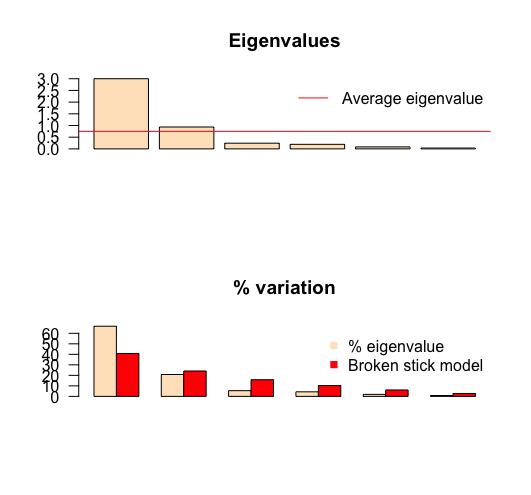
The scree plot (a) “shoulder rule” method aims to determine the point where adding another principal component does not explain much variance in comparison to previous principal components. We may identify “shoulder” on 3rd principal component. According to this method, we choose number of PCs just before “shoulder”, so 2.
Another method directly connected with scree plot method is picking a threshold of culminative variance explained by the first n PCs. The 90% rule of thumb suggests to choose q to be the smallest integer such that the q first PCs explain at least 90% of variance. According to this method I should choose 3 PCs which explain in total 93% of variance.
The broken-stick model retains components that explain more variance than would be expected by randomly dividing the variance into p parts. As can be seen in the plot, we should only choose the first component because only its variation is greater than that given by broken stick model 2.

The entries of first PC loading tells us that the first PC score is essentially the contrast between Diagonal and Bottom, Top, Right, Left. The second entries of PC loading tells us that the second PC score is essentially a contrast between Bottom, Diagonal and Top, Left, Right.


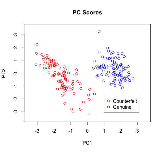
For non-standarised data, PC scores of both genuine and counterfeit banknotes form separate groups, which has little overlap. Based on this finding we may classify new banknote to be genuine, or counterfeit. The spread of PC scores of genuine banknotes is relatively small in comparison to counterfeit banknotes.
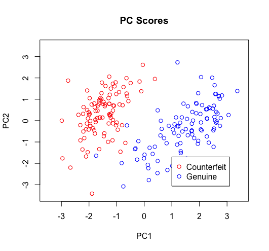
In comparison to non-standarised data, the overlap between PC scores of genuine and counterfeit groups is higher. Spread of PC Scores of both groups is also higher. The PC scores are different and there appear to be more outlier PC scores.
R code used to conduct analysis:
library(devtools)
library(factoextra)
library(easyGgplot2)
library(lattice)
library(magrittr) ## allows to write g(f(x)) as x %>% f %>% g
library(uskewFactors)
data(banknote)
?banknote ## check the help page for the dataset
names(banknote)[7]  <- 'genuine' # the 7th column says whether a banknote is genuine
summary(banknote)
X <- banknote[,-7] # the data matrix
banknote.pca <- prcomp(X, scale=FALSE)
sdPC <- banknote.pca$sdev %>% round(2) # returns the standard deviations of the PC scores.

varPC <- sdPC^2
perTotVar <- (varPC[1]+varPC[2])/sum(varPC) #Question 2

y <- c(1,2,3,4,5,6)
plot(banknote.pca, yaxt="n") #Question 1
points(y, sdPC)
plot(banknote.pca, xlab="Pricipal Component")

## ------------------------------------------------------------------------
banknote.pca$rot[,1:2] %>% round(2)

## ------------------------------------------------------------------------
banknote.pca$x[,1:2] %>% round(2)

plot(banknote.pca$x[,1], banknote.pca$x[,2],
     col=ifelse(banknote$genuine==1, "blue", "red"),
     xlab="PC1", ylab="PC2", main="PC Scores", ylim=c(-3.5,3.5),xlim=c(-3.5,3.5))

legend (1,-1.7, legend=c("Counterfeit", "Genuine"), box.lwd = 1,
       col=c("red", "blue"), pch=1)
## ------------------------------------------------------------------------
x = 1:2; y = x; names(y) <- c('a', 'b')
all.equal(x,x)
all.equal(x,y) # doesn't work since y has names
all.equal(x,y, check.attributes=FALSE) # use this version instead
all.equal(x,x+1) # answer if not equal:
all.equal(x, t(x)) ## the two quantities should be in the same format
## ------------------------------------------------------------------------
# Task f

all.equal(scale(as.matrix(banknote.pca$x[,3])),
          scale(as.matrix(X) %*% as.matrix(banknote.pca$rot[,3])), check.attributes=FALSE)

## ------------------------------------------------------------------------
# task g
all.equal(round(abs(eigen(cov(X))[[2]]),10), round(abs(banknote.pca[[2]]),10), check.attributes=FALSE)

all.equal(abs(eigen(cov(X))[[2]]), abs(banknote.pca[[2]]), check.attributes=FALSE)

## ------------------------------------------------------------------------
# task i - standarized variable PCA analysis

banknote.pca2 <- prcomp(X, scale=TRUE)

plot(banknote.pca2$x[,1], banknote.pca2$x[,2],
     col=ifelse(banknote$genuine==1, "blue", "red"),
     xlab="PC1", ylab="PC2", main="PC Scores", ylim=c(-3.5,3.5),xlim=c(-3.5,3.5))

legend (1,-1.7, legend=c("Counterfeit", "Genuine"), box.lwd = 1,
        col=c("red", "blue"), pch=1)

all.equal(cov(scale(banknote)), cor(banknote), check.attributes=FALSE)

