Time Series Model Fitting
I have chosen a time series of unemployment rate in the UK (number of people unemployed within whole labour force) recorded with monthly frequency. The data comes from the Office for National Statistics webpage and can be accessed directly: https://www.ons.gov.uk/employmentandlabourmarket/peoplenotinwork/unemployment.
I have chosen this data because it is clearly non-stationary (has non-constant variance), it exhibits changes in trends, and includes 574 observations - so that asymptotic results hold.
For that reason, this time series seems to be challenging to analyse. Most probably it will require transformations before I can fit any model.
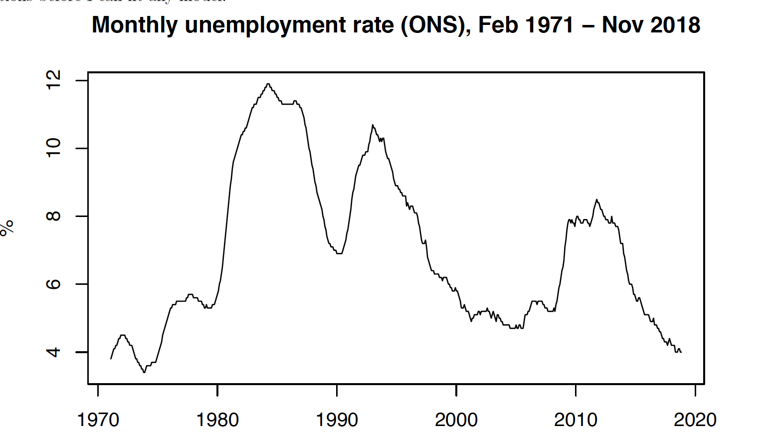
I conduct Augmented Dickey-Fuller unit root test to check if the time series is wealky stationary (that is stationary in its first two moments).
The ADF test claims that I can not reject the null hypothesis in favour of alternative hypothesis (that the time series is stationary) at any sensible significance level.
Because of that, I will transform the time-series by taking log difference. Log is a monotonic transformation which does not change the time-series (just smooth it). Difference in logs is a good approximation for growth rate, if growth rate is below 10%. As unemployment rate do not rise rapidly, I use this transformation.
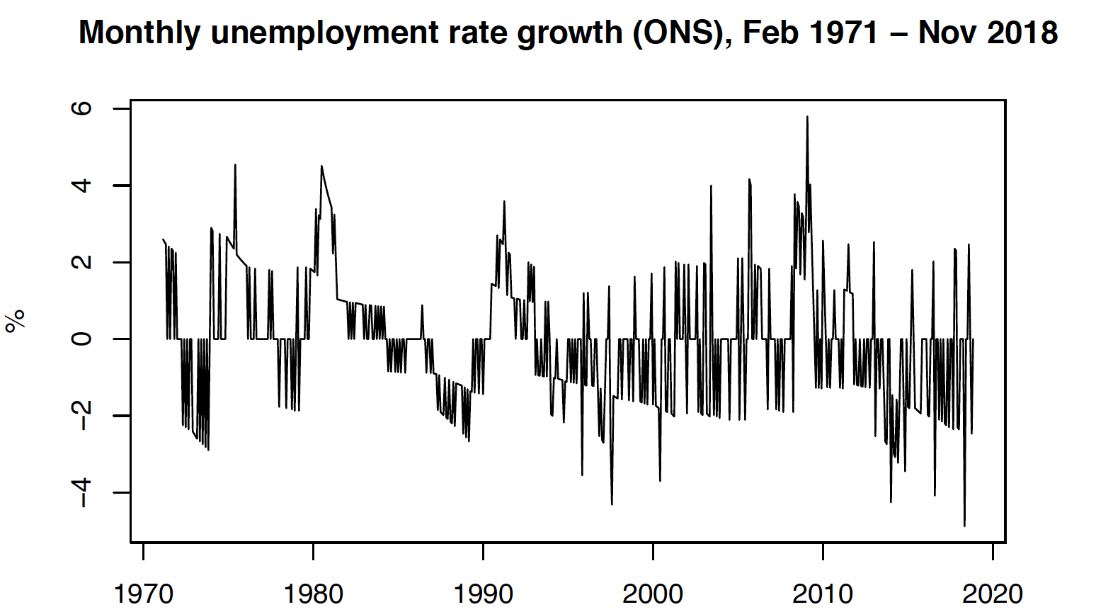
It is also necessary to check periodicity of the time-series. We may suspect some periodicity based on above plot. I would also expect unemployment rate to be periodic, as this time series is directly affected by the economic cycles.
Periodogram analysis suggests no periodicity in original time series. Although analysis suggests periodicity of 192 on growth rates, I do not take it into consideratin, because original data has no periodicity. Also peiodicity of 192 would mean that there are just 2 periods.
I proceed with analysis of this time series, as it is not white noise. acf and pacf clearly show dependency within data. Box test also reject the null hypothesis of no linear dependency at the high significance level.
I found time-series to be autoregressive process of order 5 AR(5). I established that in following steps:
-
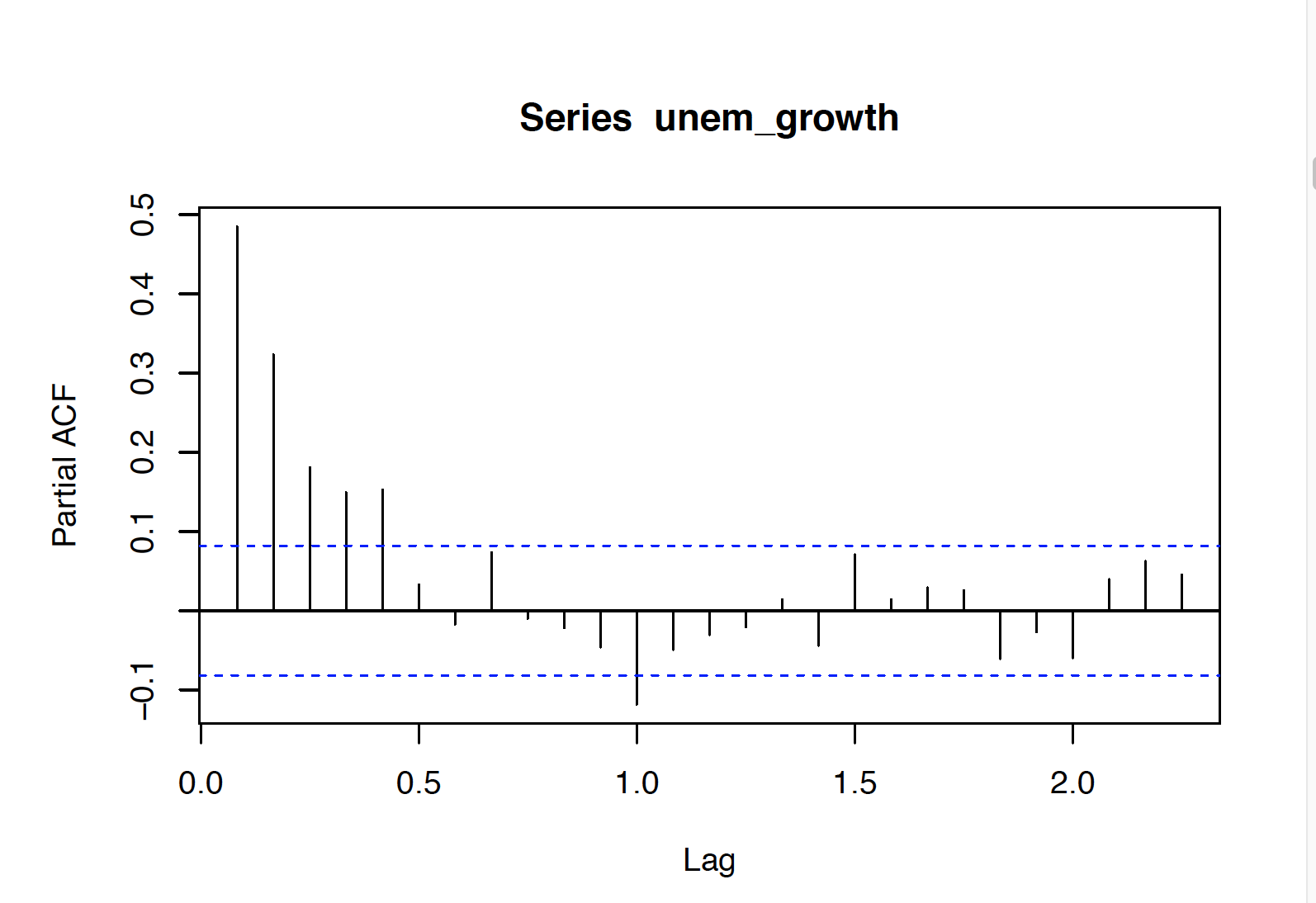
Lag selection I first specify the order using partial autocorrelation function. It suggested 5 lags. This however might be misleading, and show more lags than necessary due to correlation of later lags with each other. Next I used AIC. Akaike information criteria is a theoretical approach to lag selection. It suggests that we should select 5 lags.
-
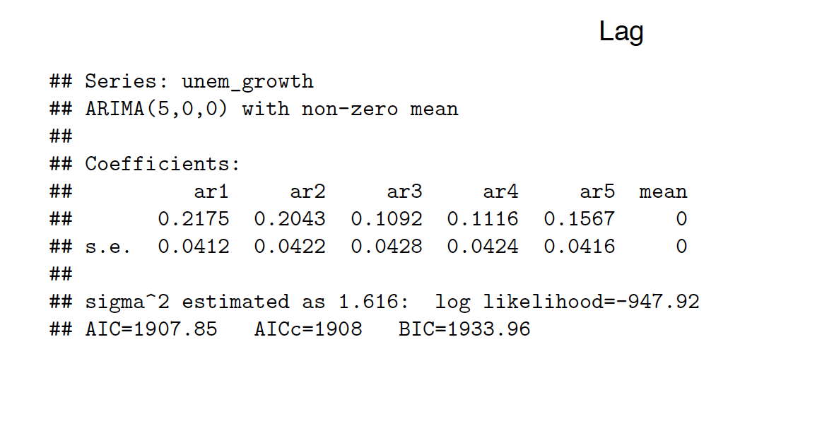
Model Fitting I fit AR(5) model. I specify AR(5) model. I supress mean to be 0, since it is not significant based on standard error. The AR coefficients are as follows: 0.2175(0.0412), 0.2043(0.0422), 0.1092(0.0428), 0.1116(0.0424), 0.1567(0.0416). Coefficients are statistically significant.
-
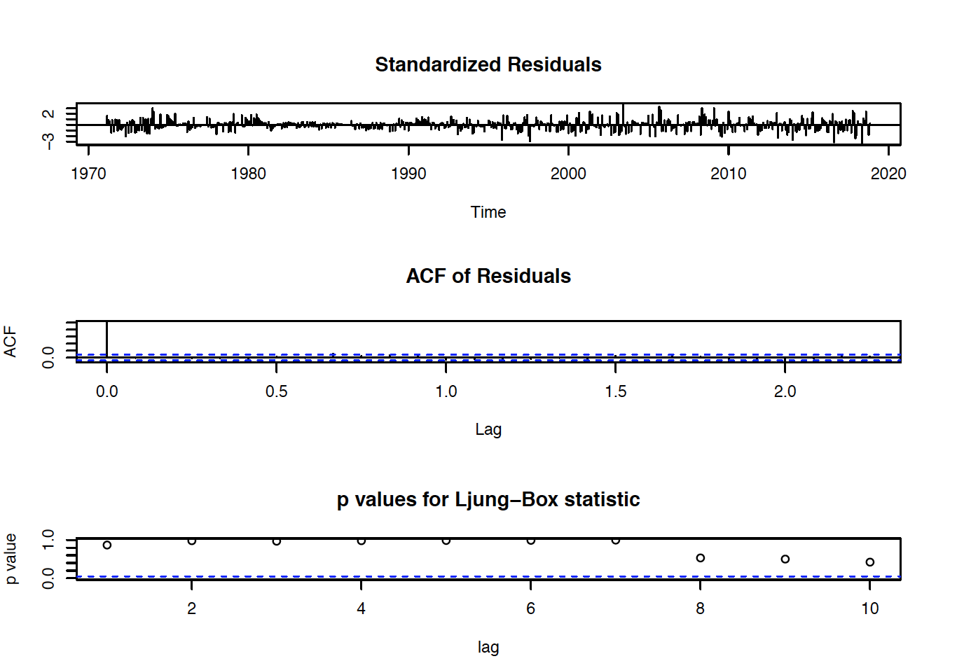
Model Validation Model AR(5) is correctly specified. Residuals of specified model are not serially correlated, acf and pacf dont show any significant lags, plot suggests constant mean. Variance of residuals is heteroskedastic, but I will not account for that as it is outside the scope of this project. Stationarity of residuals is confirmed by the Augmented DF test. I reject the null hypothesis in favour of alternative that residuals are stationary at 0.01 level. Given above facts, I assume that AR(5) is a good model, as it’s residuals are white noise.
###ARMA(p,q) Model I have chosen ARMA(1,1) model. It is the most parsimonious model, which has all coefficients significant and its residuals are white noise. The coefficients of this model are: AR(1) 0.9432(0.0178), MA(1) -0.6897(0.0351), and mean is not statistically significant, thus I set it to be 0.
The most relevant steps involve:
-
Order Specification In order to find number of lags p,q of ARMA(p,q) model, I first have checked extended autocorrelation function and tested the most parsimonious models ARMA(1,1), ARMA(1,2), ARMA(1,3)
-
Model fitting After specifying lags, I fitted the model and checked if all of the coefficients are significant. If not, I supressed them to 0.
-
Model Validation I tested if residuals of above models are white noise. If not, that violates the assumption and model is not correctly specified. In order to check if they are white noise, I ran stationarity test (ADF), check autocorrelation and partial autocorrelation functions, conducted box test and visually asess residual plot. Although ADF test rejects the null hypothesis of unit root, the variance seems heteroskedastc. I, again, will not account for that in this project but this could be fixed by fitting arch, or garch models.
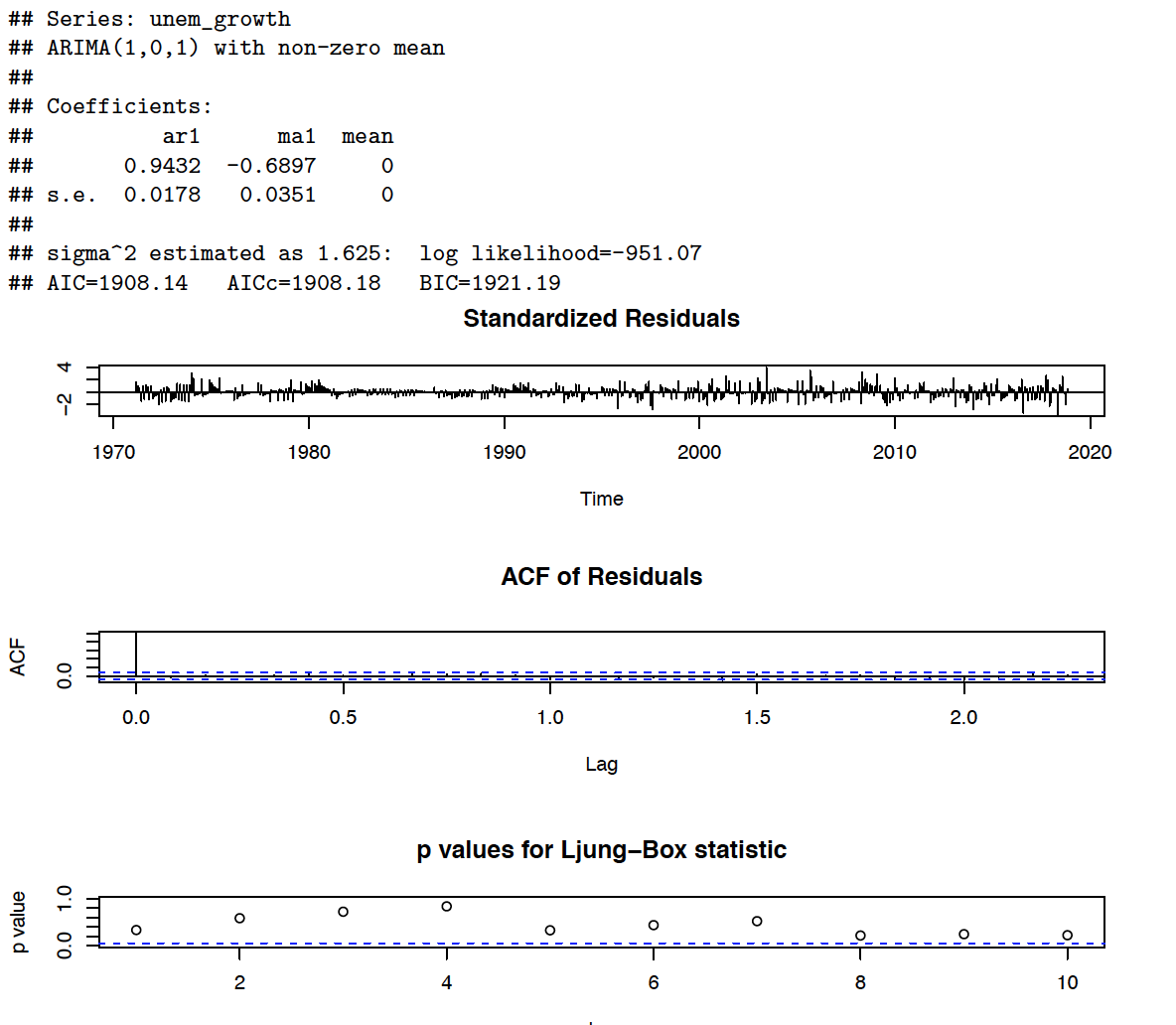
###Comparison of Models AR(5), ARMA(1,1) We can compare the performance of two selected models, AR(5) and ARMA(1,1), based on Akaike Information Criteria, Bayesian Information Criteria, Log Likelihood and adjusted R^2. For AIC and BIC model with lower score is considered to be better. In case of Log Likelihood, we want to maximise it.
Akaike Information Criteria does not indicate clearly which model performs better, as the difference in AIC is too small (0.287).
Bayesian Information Criteria indicates that ARMA(1,1) model is better, as its BIC score is lower by more than 12 points.
Higher log likelihood indicates better model. Although AR(5) has higher likelihood ratio, it s just higher by 3.
Finally, R squared and adjusted R squared (goodness of fit) is almost identical in both cases.
Based on above findings, I propose to choose ARMA(1,1) model, as difference in BIC score seems to be significant
###Root Mean Sqared Error Comparison
I computer Root mean squared error of prediction by fitting ARMA(1,1) model and AR(5) model to N-50 observations, forecasting 50 observations based on fitted models and computing root mean squared error.
I fitted exponential moving average model on N-50 parameters, with p-optimal smoothing parameter computed separately. Smoothing parameter has been obtained using optimizer defined in function HoltWinters, which minimizes MSE.
We may see that the ARMA(1,1) model has much lower mean squared error (1.69), compared to AR(5) model (1.74). However, the EMA with optimal smoothing has the lowest mean square error of 1.62.
##(iv) Checking ARMA(1,1) and AR(5) models [10 points]
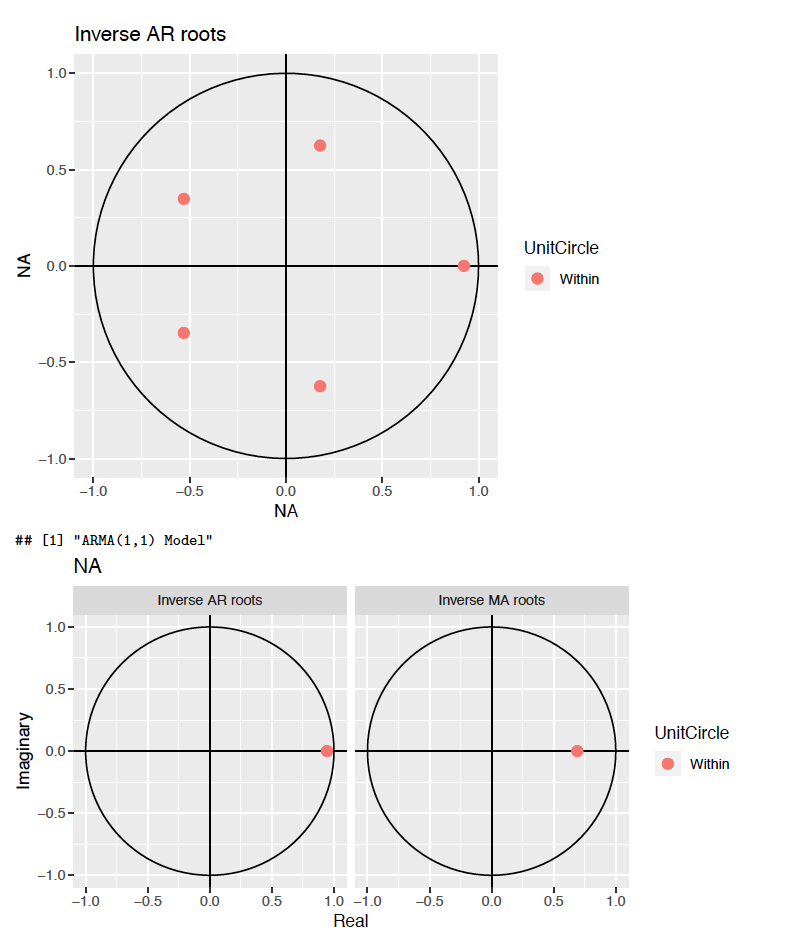
Time series is stationary if its AR roots lie outside the unit circle. Time series is invertible if its MA roots lie outside the unit circle. Pure AR models are always invertible, because they do not contain an MA component. Thus, we conclude that AR is invertible without any investigation.
Below graphs show inverses of roots of AR(5) and ARMA(1,1) models. This way, it is more compact to see if stationarity and invertability of model is true, as it’s enough to note if inverses of roots lie inside the unit root circle. We may note that all inverses of roots lie inside the unit circles. This means that AR(5) model is stationary and ARMA(1,1) model is both stationary and invertible.
V
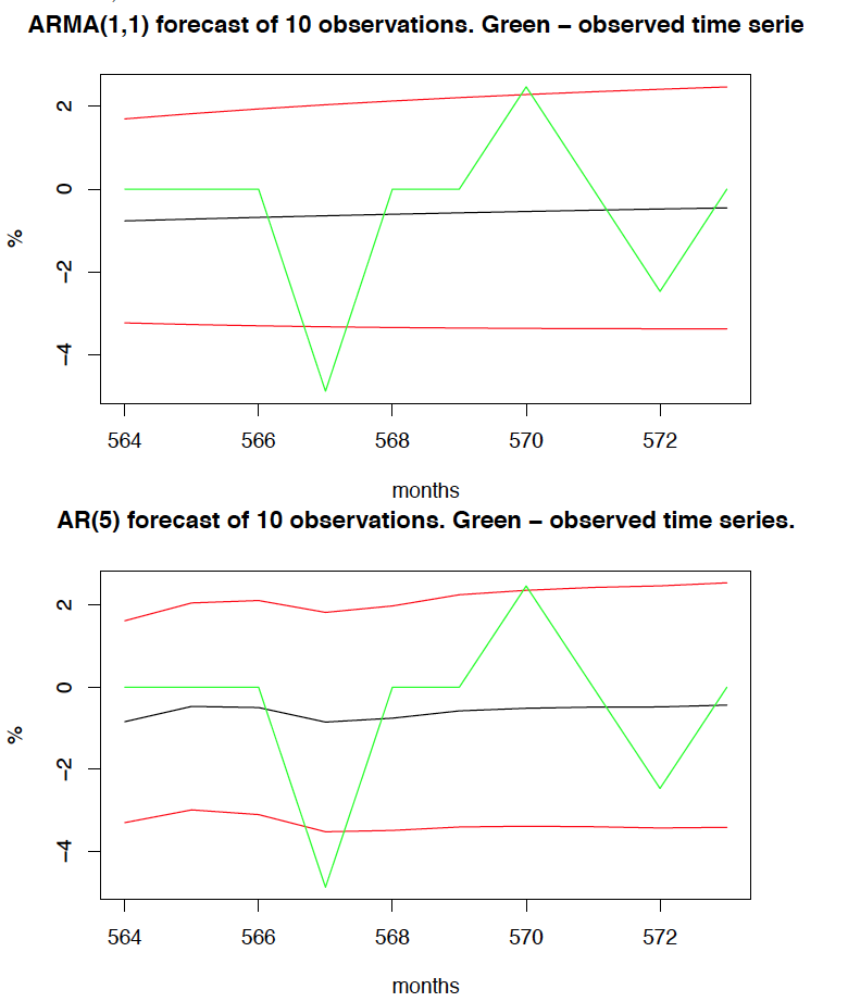
Below we may note that the forecasting based on AR(5) model is better, compared to the original series because it changes in places where original time series changes.
In general both models are not very useful to predict the movements of the time series in the short run, as we can see that both of them are very close to the mean, and quite far away from the original data.
In case of AR(5) and ARMA(1,1) model, the original time series exceeds the 95% confidence interval twice. In order to get more accurate predictions, we would either need more data, or make the forecast shorter (thus more accurate).
R code used to conduct analysis:
##Question (i)
unem_data <- read.csv(file="series-200219.csv")
unem_data <- unem_data$unempl
unem_ts <- ts(unem_data, frequency = 12, start=c(1971,2))
plot(unem_ts, xlab="", ylab="%")
title("Monthly unemployment rate (ONS), Feb 1971 - Nov 2018")
library(tseries)
adf.test(unem_ts)
unem_growth <- diff(log(unem_ts))*100
acf(unem_growth) # Not white noise
adf.test(unem_growth)
plot(unem_growth, xlab="",ylab="%")
title("Monthly unemployment rate growth (ONS), Feb 1971 - Nov 2018")
b_test1=Box.test(unem_growth, lag=max(log(length(unem_data)),5)) #Reject null at high level, - no white noise
library(TSA)
prd = periodogram(unem_data);
ord = order(-prd$spec);
d = cbind(prd$freq[ord],prd$spec[ord]);
head(d);
period = 1/d[1,1]; #period detected by periodogram is one over one number
period # Did not detect any period (576)

##Question (ii)
library(tseries)
library(TSA)
library(forecast)
library(tseries)

acf(unem_growth)
pacf(unem_growth) # Suggests order 5
ar(unem_growth,order=5)
ar(unem_growth)$aic #selected order 5
M = Arima(unem_growth,order = c(5,0,0), fixed = c(NA,NA,NA,NA,NA,0))
M
res = M$residuals
plot(res)
acf(res)
pacf(res)
Box.test(res,lag = max(log(length(unem_growth)),10), fitdt=5) #independent (dont reject the null)
adf.test(res) # reject the null at the 0.01< level, stationary
#All conditions for the white noise are met

##Question (iii)

eacf(unem_growth)
K=Arima(unem_growth,order=c(1,0,1), fixed=c(NA,NA,0));
K
res_1 = K$residuals
plot(res_1)
acf(res_1)
pacf(res_1)
Box.test(res_1,lag = max(log(length(unem_growth)),7), fitdf = 2) #independent (dont reject the null)
adf.test(res_1) # reject the null at the 0.01< level, stationary
#All conditions for the white noise are met

L=Arima(unem_growth,order=c(1,0,2), fixed=c(NA,NA,NA,0))
L #MA(2) coefficient is not significant
res_1 = M$residuals
plot(res_1)
acf(res_1)
pacf(res_1)
Box.test(res_1,lag = max(log(length(unem_growth)),8), fitdf=3) #independent (dont reject the null)
adf.test(res_1) # reject the null at the 0.01< level, stationary
# All conditions for the white noise are met

N=Arima(unem_growth,order=c(1,0,3)) #not significanr AR2 and AR3 coefficient
N
res_2 = N$residuals
plot(res_2)
acf(res_2)
pacf(res_2)
Box.test(res_2,lag = max(log(length(unem_growth)),9), fitdf=4) #independent (dont reject the null)
adf.test(res_2) # reject the null at the 0.01< level, stationary
# All conditions for the white noise are met

# Comparing Akaike Information Criteria, difference doesnt seem significant
K$aic
M$aic

# Comparing Bayesian Information Criteria, AR(5) model seems to be inferior to ARMA(1,1) model
K$bic
M$bic

# Comparing log likelihood -  the higher the better - AR(5) model performs better - but may be not statistically significant
K$loglik
M$loglik

Rsquared_K = 1 - sum(K$residuals^2)/sum((unem_growth-mean(unem_growth))^2)
Rsquared_M = 1 - sum(M$residuals^2)/sum((unem_growth-mean(unem_growth))^2)


T = length(unem_growth);
adjRsquared_K = 1 - (T-2-1)/(T-2*2-1)*(sum(K$residual^2)/sum((unem_growth-mean(unem_growth))^2))
adjRsquared_M = 1 - (T-5-1)/(T-2*5-1)*(sum(M$residual^2)/sum((unem_growth-mean(unem_growth))^2))
print(c(Rsquared_K,Rsquared_M))

unem_growth_1 <- unem_growth[1:523]
K1 <- Arima(unem_growth_1,order = c(1,0,1))
predictions_1 = forecast(K1,50)
predictions_1 = as.numeric(unlist(predictions_1$mean))

library(Metrics)
print("RMSE of ARMA(1,1)")
rmse(unem_growth[524:573], predictions_1)

M1 <- Arima(unem_growth_1,order = c(5,0,0))
predictions_2 = forecast(M1,50)
predictions_2 = as.numeric(unlist(predictions_2$mean))

print("RMSE of AR(5)")
rmse(unem_growth[524:573], predictions_2)

library(tseries)
library(TTR)
library(forecast)

HoltWinters(unem_growth, beta=FALSE, gamma = FALSE)
W <- EMA(unem_growth[0:523],ratio=0.2717976,type=e)
predictions_3 <- forecast(W, 50)
predictions_3 = as.numeric(unlist(predictions_3$mean))

print("RMSE of EMA with p optimal smoothing parameter)")
rmse(unem_growth[524:573], predictions_3)

##Question (iv)

library(forecast)
autoplot(M)
autoplot(K)

##Question (v)


unem_growth_10 <- unem_growth[1:564]
GM <- Arima(unem_growth_10,order = c(1,0,1), fixed=c(NA,NA,0))
PG <- predict(GM,10)

c=PG$pred+1.96*PG$se
d=PG$pred-1.96*PG$se
tspl=cbind(PG$pred, c,d,unem_growth[565:574])
ts.plot(tspl,gpars=list(col=c("black","red","red","green")))

unem_growth_10 <- unem_growth[1:564]
GM <- Arima(unem_growth_10,order = c(5,0,0), fixed=c(NA,NA,NA,NA,NA,0))
PG <- predict(GM,10)

c=PG$pred+1.96*PG$se
d=PG$pred-1.96*PG$se
tspl=cbind(PG$pred, c,d,unem_growth[565:574])
ts.plot(tspl,gpars=list(col=c("black","red","red","green")))

