Fitting ARMA and GARCH to S&P500 Volume Time Series
I have chosen a time series related to S&P500 which includes 500 companies with the biggest capitalisation listed on NYSE, NASDAQ. I focus on volume (number of stocks traded every mounth) of stock traded on S&P500 (between Jul 2000-Mar 2019). The data comes from the Yahoo Finance webpage and can be accessed directly: https://finance.yahoo.com.
I have chosen this data because it is clearly non-stationary as it has positive trend and non-constant variance. The time series includes 190 observations - so that asymptotic results hold. Furthermore, time series has a huge variance around the 2008 downturn. Data are recorded with monthly frequency and units are numbers of stocks.
Because of heteroscedasticity and change in trend, the time series most probably will require transformations before I can fit any model.
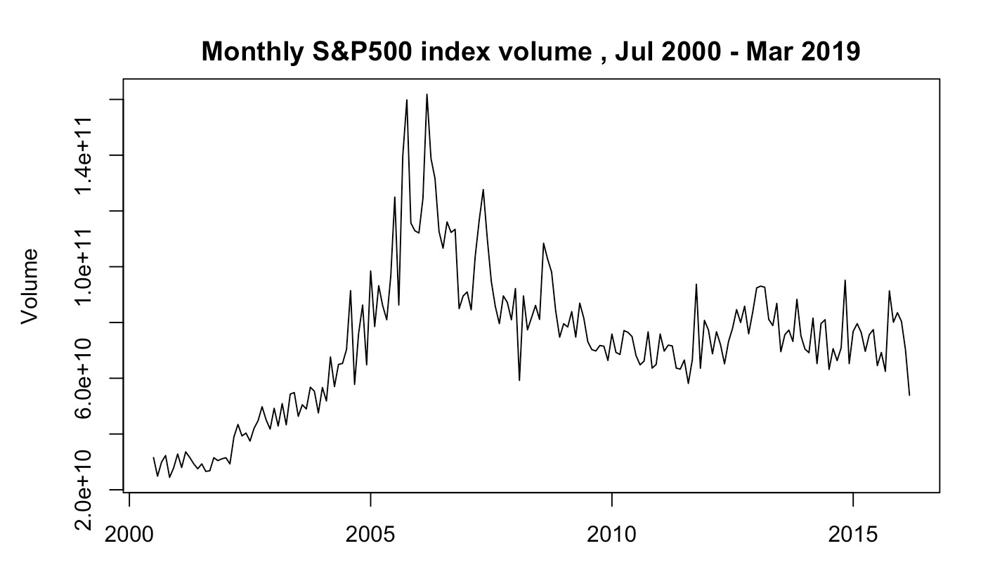
I conduct Augmented Dickey-Fuller unit root test to check if the time series is wealky stationary (that is stationary in its first two moments). This is necessary due to possible spurious correlation problem highlighted by Granger.
The ADF test claims that I can not reject the null hypothesis in favour of alternative hypothesis (p value is 0.74) (can’t reject the null that the time series is stationary) at any sensible significance level (the mean is clearly non constant and variance varies with time).
Because of that, I will transform the time-series by taking log difference. Log is a monotonic transformation which does not change the time-series (just smooths it).
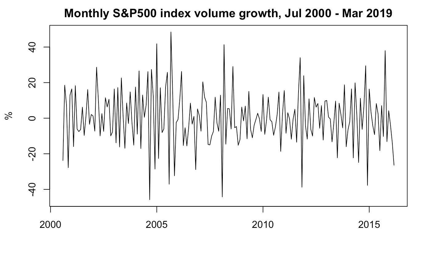
Although the ADF test rejects the null hypothesis (so our transformed time series is stationary), the time series is also clearly heteroscedastic. We may note that it has relativel low variance between 2000 and 2004, and the variance increases rapidly during 2005, and falls again. This phenomenon repeats at least 4 times. Thus, conditional heteroscedasticity occurs.
Periodogram analysis suggests no periodicity in original time series.
I proceed with analysis of this time series, as it is not white noise. acf and pacf clearly show dependency within data. Box test also reject the null hypothesis of no linear dependency at the high significance level.
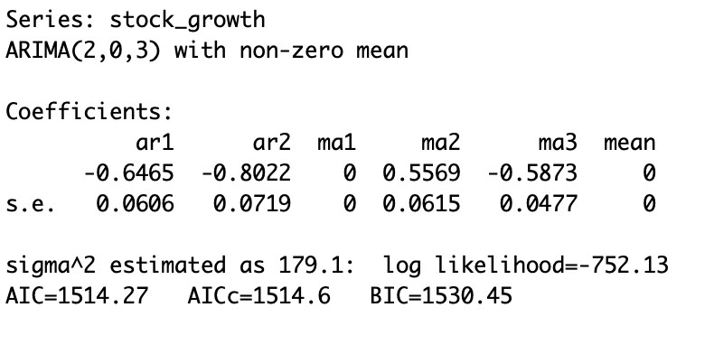
I have chosen ARMA(2,3) model. It is the most parsimonious model, which has all coefficients significant and its residuals are white noise.The MEAN and MA(1) coefficients are not statistically significant, thus I set it to be 0.
The most relevant steps involve:
-
Order Specification: In order to find number of lags p,q of ARMA(p,q) model, I first have checked extended autocorrelation function and tested the most parsimonious models ARMA(1,1), ARMA(1,2), ARMA(3,2)
-
Model fitting: After specifying lags, I fitted the model and checked if all of the coefficients are significant. If not, I supressed them to 0.
-
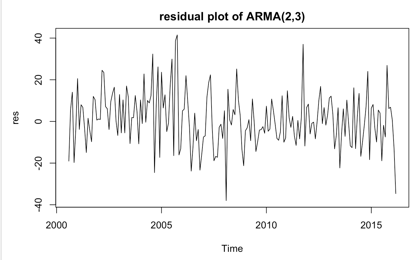
Model Validation: I tested if residuals of above models are white noise. If not, that violates the assumption and model is not correctly specified. In order to check if they are white noise, I ran stationarity test (ADF), check autocorrelation and partial autocorrelation functions, conducted box test and visually asess residual plot. Although ADF test rejects the null hypothesis of unit root, the variance seems heteroscedastc. Residuals don’t have any significant early autocorrelation.
Heteroscedasticity and fitting Arch and Garch models
Garch and Arch models are appropriate, because tests based on squared residuals of above ARMA(2,3) model, such as acf and pacf, clearly show significant correlation at some lag orders. Similarly, the box test based on squared residuals rejects the null hypothesis, which means that residuals are not a white noise. When residuals are plotted, we may clearly see some heteroscedasticity, which contradicts the standard assumtions of well defined ARMA(p,q) model.
Although augmented Dickey Fuller test shows that the residuals are stationary, above analysis shows that we need to account fot heteroscedasticity by fitting Arch or Garch model together with ARMA(2,3).
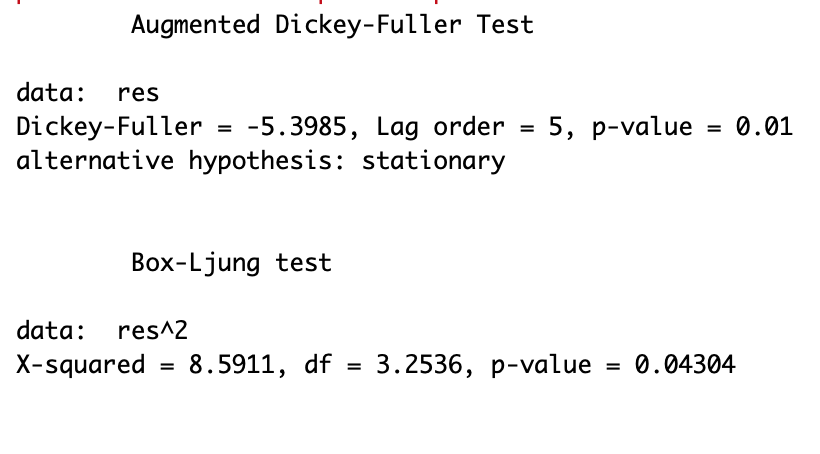
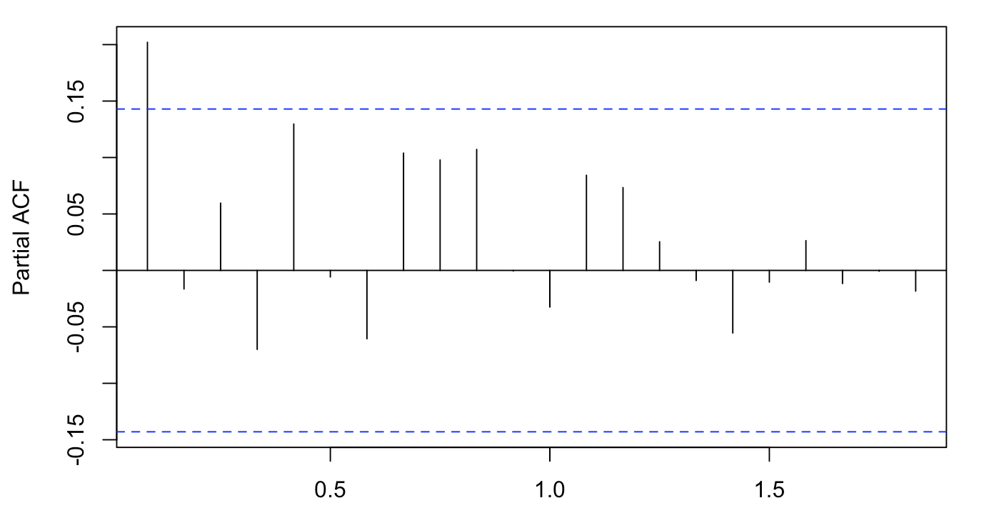
In order to account for this heterogenity in residuals, I attempt to fit everal Garch and Arch models. Overall, I test arch(1), arch(2), arch(3), Garch(1,1), Garch(2,1), Garch(1,2). The fitted Arch(1) seems account for heteroscedasticity most accuretally (based on significance of coefficients and model validation), thus I will describe it in detail.
Fitted Arch model has MEAN mu with non-significant coefficient, which meanst I can’t reject the null hypothesis that it’s zero. That is required by our model. While omega coefficient is significant, the alpha coefficient is borderline significant (its p-value is 0.08). However, when I tried to fit arch model of higher order, both omega and aplha_1 were significant, while remaining alpha were not significant. Thus, I specify arch(1) model and assume it fits data well.
The fitted Arch model has the following form: (\sigma)(^2) = (\alpha)(0)+(\alpha)(1)a(^2)(t-1)
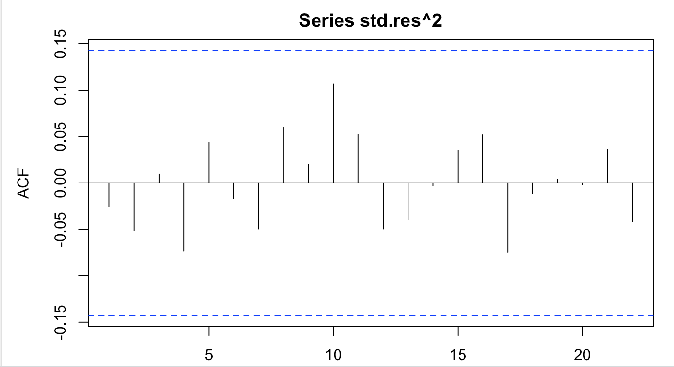
Next, I analyse the standarised residuals. The acf of standarised residuals and acf of squared standarised residuals don’t display any significant correlations (just one borderline case). The Box test of standarised residuals and standarised squared residuals do not reject the null hypothesis, which means that in both cases autocorrelation up to lag 10 is equal to 0.
Above analysis concludes that Arch(1) is a sufficient model, and diagnostic statistics show that it captures volatility visible within residuals of initial ARMA(2,3) model.
The only not satisfactory aspect is borderline significant autocorrelation of lag 13, but it disappears later when I fit ARMA and ARCH together. Details of arch(1) model are displayed in appendix.
Fitting ARMA(2,3) and Arch(1) models
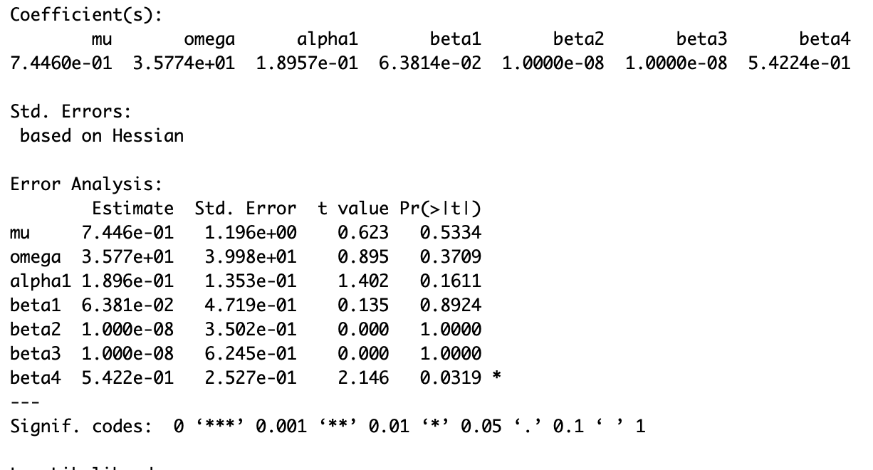
Next, I proceed to fitting ARMA(2,3) and Arch(1) model together.The model details are displayed below. We may note that MA(1) and ‘mean’ coefficients are not significant. Also alpha1 is borderline significant, however as I argued above, it is not a problem during our analysis. Also shape coefficient is not significant.
Thus, when I fit the model, I exclude mean and shape (force it to be fixed numbers). Our model then becomes very significant in most of the cases. MA(1) becomes borderline significant (but it’s not a problem) and alpha1 is borderline significant (but as explained above, it fits the model well). We should check if this model is sufficuent during model validation.
Model Validation ARMA(3,2) and Arch(1)
We may note that residuals of model specified above behave even better than in case of fitting Arch model on residuals of ARMA(2,3) model. Back then, there was one borderline lag. Below, I displayed the acf of residuals and squared residuals of above model. Non of the lag is even borderline significantly autocorrelated.
The box test does not reject the null hypothesis at a high level, meaning that residuals of above model are white noise both in case of residuals and squared residuals.
Agumented Dickey Fuller test rejects the null in favour of alternative hypothesis that the residuals are stationary at a high significance level (<0.01). This is also best model as measured by and AIC and BIC.
Fitted Volatility Function
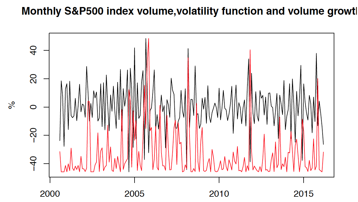
I have displayed volatility function and volume growth (stationary time series) below. We may clearly note that there are 4 significant volatility peaks. One in 2006, 2008, 2013 and 2016. Clearly, the biggest volatility peaks are between 2006 and 2008. This is linked to the 2008 downturn, when the stock market was vary volatile. Many market players probably traded a lot of stock within S&P500 index, in order to sell their stock (or buy on low prices).
When volatility function is plotted against T-1 stationary time series, it is visible that volatility peaks occur after the abnormally high variance of the volume growth. This is in line with our predictions, as these extreme values need to be accounted for during fitting the arch model.
EGARCH and GARCH-M
EGARCH model accounts for assymetric reaction of conditional variance to positive and negative shocks. In finance the positive shock have usually lower impact than negative shocks. This is the consequence of loss aversion, as market players are more hurt by loosing money than by gaining equivalent amount. The main aim of EGARCH model is to reporoduce leverage effect. Based on residual plot of residuals ARMA(2,3) model, there is no assymetric behaviour of growths and fall in volume of traded stocks.
GARCH-M model is introducing the risk premium. The general idea is that the more volatile security is, the more risk premium it requires. This series is unrelated to the examined time series (volume of traded stocks), thus I would expect that the fitted GARCH-M would either give bad results, or good fit would be a coincidence.
To sum up, as I fit the amount of traded stock on S&P500 (Volume), I would not expect it to have a strong EGARCH or GARCH-M effects. Maybe EGARCH could be more appropiate, because usually when stock are traded more, the market reacts much more volatile than when volumes traded are low. I decided to proceed with EGARCH model, as it has more significant coefficients and seems to fit data better.
EGARCH model together with ARMA(2,3) model have non-significant mu, AR(1), omega, alpha1, beta1, gamma1 coefficients. This means that this model is not suitable to account fot heteroscedasticity in residuals of our ARMA(2,3) model. Compared to GARCH-M model, it has more significant AR and MA coefficients. Overall, non of this model provides a better fit to the ARMA+ARCH model discussed in previous question.
stock_data <- read.csv(file="^GSPC.csv")
#print(stock_data)
stock_data <- stock_data$Volume
stock_ts <- ts(stock_data, frequency = 12, start=c(2000,7))
plot(stock_ts, xlab="", ylab="USD")
title("Monthly S&P500 index volume , Jul 2000 - Mar 2019")

library(tseries)
#adf.test(stock_ts)
stock_growth <- diff(log(stock_ts))*100
#pacf(stock_growth) # Not white noise
#adf.test(stock_growth)
plot(stock_growth, xlab="",ylab="%")
title("Monthly S&P500 index volume growth, Jul 2000 - Mar 2019")
#b_test1=Box.test(stock_growth, lag=max(log(length(stock_growth)),5)) #Reject null at high level, - no white noise
#print(b_test1)

library(TSA)
#prd = periodogram(stock_ts);
#ord = order(-prd$spec);
#d = cbind(prd$freq[ord],prd$spec[ord]);
#head(d);
#period = 1/d[1,1]; #period detected by periodogram is one over one number
#period # Did not detect any periodicity

library(tseries)
library(TSA)
library(forecast)
library(tseries)


#acf(stock_growth) # Early dependance suggests order 5
#ar(stock_ts,order=5)
#ar(stock_growth)$aic #selected order 5
#eacf(stock_growth)
M = Arima(stock_growth, order = c(2,0,3), fixed = c(NA,NA,0,NA,NA,0))
print(M)
#tsdiag(M)
res = M$residuals
#acf(res) #It has no significant early correlation
#pacf(res) #It has no significant early correlation
plot(res) #Still some visible heteroskedasticity


adf.test(res) # reject the null at the 0.01< level, stationary

# acf(res^2)
pacf(res^2)
Box.test(res^2,lag = log(length(stock_growth),5),type = "Ljung")
plot(res)
# All conditions for the white noise are met

library(fGarch)
mARCH = garchFit(~garch(1,0),res,trace=F)
summary(mARCH)
# mARCH = garchFit(~garch(2,0),res,trace=F)
# summary(mARCH)
# mARCH = garchFit(~garch(3,0),res,trace=F)
# summary(mARCH)
# mARCH = garchFit(~garch(1,1),res,trace=F)
# summary(mARCH)
# mARCH = garchFit(~garch(1,2),res,trace=F)
# summary(mARCH)
std.res = mARCH@residuals/mARCH@sigma.t
#plot(std.res,type="l")
acf(std.res)
acf(std.res^2)
Box.test(mARCH@residuals/mARCH@sigma.t,lag=10,fitdf=1,
         type="Ljung-Box")
Box.test(std.res^2,lag=10,fitdf=1,
         type="Ljung-Box")

mARCHt = garchFit(formula = ~arma(2,3)+garch(1,0),data = stock_growth,
                  cond.dist="std",trace=F)

summary(mARCHt)


std.res = mARCHt@residuals/mARCHt@sigma.t
#plot(std.res,type="l")
acf(std.res)
acf(std.res^2)
Box.test(std.res,lag=10,fitdf=5,
         type="Ljung-Box")
Box.test(std.res^2,lag=10,fitdf=5,
         type="Ljung-Box")
adf.test(std.res)

#plot(mARCHt@sigma.t,stock_growth,xlab="Fitted Volatility",ylab="Growth", type='l)
#plot(,type="l")mARCHt@sigma.t
#lines(mARCHt@sigma.t,col="blue",lwd=3)
plot(stock_growth,type="l", xlab = "", ylab = "%")
par(new = TRUE)
plot(mARCHt@sigma.t, type="l", col="red", axes=FALSE,xlab = "", ylab = "")
title("Monthly S&P500 index volume,volatility function and volume growth")

T = length(stock_growth)

plot(stock_growth[2:T],type="l", xlab = "", ylab = "%")
par(new = TRUE)
plot(mARCHt@sigma.t, type="l", col="red", axes=FALSE,xlab = "", ylab = "")
title("Monthly S&P500 index volume,volatility function and volume growth")

library(rugarch)
plot(res)
spec = ugarchspec(variance.model = list(model = "eGARCH",garchOrder = c(1,1)),
                  mean.model = list(armaOrder = c(2,3)),
                  distribution.model = "norm");
eGARCH = ugarchfit(stock_growth,spec = spec,solver="hybrid");
print(eGARCH)
spec = ugarchspec(variance.model = list(model = "sGARCH",garchOrder = c(1,1)),
                  mean.model = list(armaOrder = c(2,3),archm = TRUE),
                  distribution.model = "norm");
GARCHM = ugarchfit(stock_growth,spec = spec);
print(GARCHM)

library(rugarch)

spec = ugarchspec(variance.model = list(model = "eGARCH",garchOrder = c(1,1)),
                  mean.model = list(armaOrder = c(2,3)),
                  distribution.model = "norm");
eGARCH = ugarchfit(stock_growth,spec = spec,solver="hybrid");
print(eGARCH)
spec = ugarchspec(variance.model = list(model = "sGARCH",garchOrder = c(1,1)),
                  mean.model = list(armaOrder = c(2,3),archm = TRUE),
                  distribution.model = "norm");
GARCHM = ugarchfit(stock_growth,spec = spec);
