Time Series Forecasting with Deep Learning

from pandas import read_csv
from pandas import Series

# Load the data from the file
data = read_csv('./pollution.csv', header=0)
# Print the summary statictics of each variable
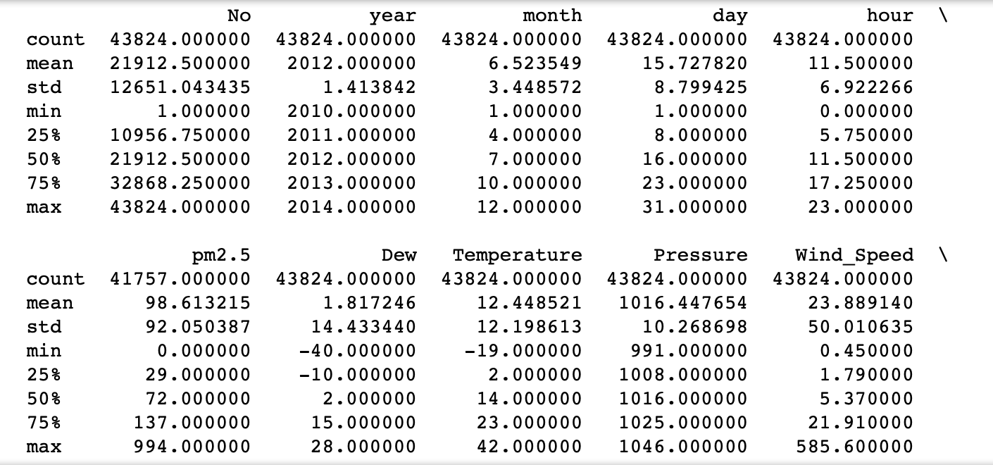
print(data.describe())

# Dropping all the unnecessary columns: index and time related
data=data.drop(columns='No')
data=data.drop(columns='year')
data=data.drop(columns='month')
data=data.drop(columns='day')
data=data.drop(columns='hour')

# Replacing the missing values with mean of the parameters, another way to tackle missing values is its removal,
# however this would lead to removing more than 2000 observations, which would cause irregularity in the time series
data.fillna(data.mean(), inplace=True)

# I plot all the numerical variables over time
plt.plot(data['Dew'])
plt.draw()
plt.figure()
plt.plot(data['pm2.5'])
plt.draw()
plt.figure()
plt.plot(data['Temperature'])
plt.draw()
plt.figure()
plt.plot(data['Pressure'])
plt.draw()
plt.figure()
plt.plot(data['Wind_Speed'])
plt.draw()
plt.figure()
plt.plot(data['Snow'])
plt.draw()
plt.figure()
plt.plot(data['Rain'])
plt.draw()
plt.figure()

# All plotted values shows clear periodicity and some regularities, which are likely to be detected by Neural Network
# These regularities could be exploited especially by LSTM layers with long periods of memory
# Plot of pollution is very volatile, it exhibits heteroskedasticity and clusters of peaks

from sklearn import preprocessing
from keras.utils.np_utils import to_categorical
from keras.models import Sequential
from keras.layers import LSTM, Dense, Activation, Dropout

# I first need to convert non-numerical variable 'wind direction' to numerical
# in order to feed it to neural network. To do so, I assign number 1 to 'SE',
# 2 to 'cv', assuming '2' is a SW, 3 to NW, and 4 to NE
Wind_Direction=[]
for i in range(len(data['Wind_Direction'])):
    if data.iloc[i,4]=='SE':
        Wind_Direction.append(1)
    elif data.iloc[i,4]=='cv':
        Wind_Direction.append(2)
    elif data.iloc[i,4]=='NW':
        Wind_Direction.append(3)
    elif data.iloc[i,4]=='NE':
        Wind_Direction.append(4)
    else:
        print("error")

# Replacing wind direction variable with its numerical values
data['Wind_Direction']=Wind_Direction
data1=data

# Shifting pollition variable by 1 hour (to get past weather data and current polution)
# and replacing missing values with mean of the column
pollution=data['pm2.5'].shift(-1)
#data['pm2.5']=data['pm2.5'].shift(-1)
data.fillna(data.mean(), inplace=True)
pollution.fillna(pollution.mean(), inplace=True)
# This part - I prepare the label data by transforming it to array, creating 2nd timension
# to feed to NN, and splitting beteen test and train and normalising
pollution=np.array(pollution) # declare it as an array
pollution=pollution.reshape(-1, 1) # need to reshape it to 2 dimensions to pass it to StandardScaler()
label_train=np.array(pollution[0:35059]) # split between train and test labels
label_test=np.array(pollution[35060:])
label_test1=label_test # Copy labels in its original form before preprocessing
scaler1 = preprocessing.StandardScaler().fit(label_train) # fitting standarisation
label_train=scaler1.transform(label_train) # preprocessing train labels
scaler2 = preprocessing.StandardScaler().fit(label_test) # fitting the standarisation
label_test=scaler2.transform(label_test) # transforming test labels


# Preparing other data, used to predict pollution. I first normalise these data, split it to test and train
scaler = preprocessing.StandardScaler().fit(data) # fitting transformation to data
data=scaler.transform(data) # transforming data which we will feed to neural network
data_train=np.array(data[:35059]) # splitting training data
data_test=np.array(data[35060:]) # splitting testing data

# I reshape input to be 3D [samples, timesteps, features], so that I can pass it to RNN
train_X = data_train.reshape((data_train.shape[0], 1, data_train.shape[1]))
test_X = data_test.reshape((data_test.shape[0], 1, data_test.shape[1]))

from keras.models import Sequential
from keras.layers import LSTM, Dense, Activation, Dropout
from pandas import DataFrame, concat
import matplotlib.pyplot as plt

# Setting random.seet to make sure data is reproductible
np.random.seed(42)
# Setting one LSTM layer, one dense layer
# fiting the NN with train data and labels defined above. Defining
model = Sequential()

model.add(LSTM(50, input_shape=(train_X.shape[1], train_X.shape[2])))
model.add(Dense(1))
model.compile(loss='mae', optimizer='adam')
history = model.fit(train_X, label_train, epochs=40,
            batch_size=72, validation_split=0.1,
            verbose=2, shuffle=False)

# plot the valuarion loss and training loss
plt.plot(history.history['loss'], label='train')
plt.plot(history.history['val_loss'], label='test')
plt.legend()
plt.show()

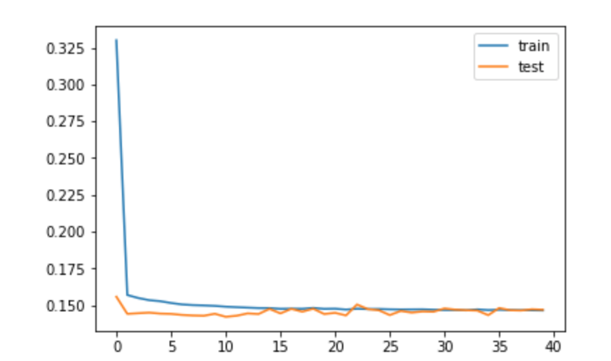
# The training loss and valuation loss converge very quickly to its lowest values
# We could stop after 15 epoch, since there is not significant gain of accuracy further
# Both loss and valuation loss are very low, below 0.15 level
# This means that the neural network is very efficient for time series prediction.
# The possible reason for that is that we have t-1 pollution in input, data is high frequency,
# thus in most cases we are able to predict the volatility of the time series really well.
# When I tried to ommit the variable 'pollution(t-1)', the prodictions were much less accurate and
# didn't capture the volatility of time series to the same extent as in below model. These predictions
# were much closer to the mean, however to some extent volatility was still captured.

from sklearn.metrics import mean_squared_error
from math import sqrt

# I transform the prediction and training label to its original dimension
alpha=scaler2.inverse_transform(label_test)

# I predict data based on trained model
beta=model.predict(test_X)
beta=scaler2.inverse_transform(beta)
print('The root mean squared error of predicted vs actual valies is is:', round(sqrt(mean_squared_error(label_test1, beta)),2))

plt.plot(alpha, label='real values')
plt.plot(beta, label='predictions')
plt.legend()
plt.show()

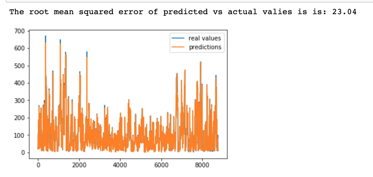
# We may note that the root mean squared error is very low 23.04 for this amount of observations
# The plot shows that the predicted time series fits almost perfectly the original time series, this is the case
# because we have lots of observations, and the model just predict t+1 observation (short forecast), so the accuracy is quite high.
# However, when we remove the shifter lagged pollution from the input data, the high variablility is not captured
# by the model. This means, that the lagged pollution is the main variable contributing to accuracy of predictions
# within this LSTM network.

from pandas import DataFrame, concat

# Setting up another model, by adding 2 LSTM layers, and 2 dropout layers, and leaving other factors the same as in above network

model = Sequential()

model.add(LSTM(50, input_shape=(train_X.shape[1], train_X.shape[2]), activation='relu', return_sequences=True))
model.add(Dropout(0.5))

model.add(LSTM(50,  activation='relu'))
model.add(Dropout(0.5))

model.add(Dense(1))
model.compile(loss='mae', optimizer='adam')

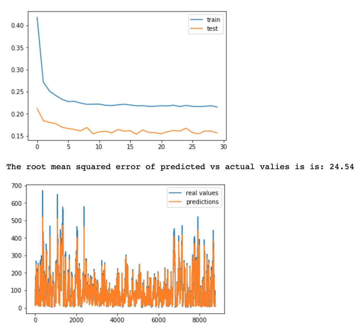
history = model.fit(train_X, label_train, epochs=30, batch_size=72, validation_split=0.1, verbose=2, shuffle=False)

# plot relevant accuracy graphs, showing train and val loss
plt.plot(history.history['loss'], label='train')
plt.plot(history.history['val_loss'], label='test')
plt.legend()
plt.show()

# Predicting output of testing data
beta=model.predict(test_X)
beta=scaler2.inverse_transform(beta)

print('The root mean squared error of predicted vs actual valies is is:', round(sqrt(mean_squared_error(label_test1, beta)),2))

plt.plot(alpha, label='real values')
plt.plot(beta, label='predictions')
plt.legend()
plt.show()

# In the case of more complicated model, consisting of dropout layers (for better generasability) and
# 2 LSTM layers, the loss (validation and testing) is higher (0.20 vs 0.15 in previous model).
# I believe that the main contributor is droupout layer. However, thanks to dropout layer,
# I would expect RMSE of testing data to be lower. In this case RMSE is higher (24.54 vs 23.04) than in case
# of more simple model with 1 LSTM layer and no dropout layer. Thus model 1 is preffered. Changing the activation
# functions, adding more dropout layers, changing epoch/bath don't decrease the RMSE

# I attach the lagged values of pollution using for loop, which then relate to the pollution over the last 3 days
# 3 days = 72 hours, thus I iterate by 1 in range 72 to 1.

# I append to the variables values of variables from the past. to predict polution at time t, I consider
# all the variable values between t-72 and t-1
for i in range(72, 1, -1):
    data1['pol',i]=data2['pm2.5'].shift(i)

for i in range(72, 1, -1):
    data1['dew',i]=data2['Dew'].shift(i)

for i in range(72, 1, -1):
    data1['temp',i]=data2['Temperature'].shift(i)

for i in range(72, 1, -1):
    data1['press',i]=data2['Pressure'].shift(i)

for i in range(72, 1, -1):
    data1['wd',i]=data2['Wind_Direction'].shift(i)

for i in range(72, 1, -1):
    data1['ws',i]=data2['Wind_Speed'].shift(i)

for i in range(72, 1, -1):
    data1['sno',i]=data2['Snow'].shift(i)

for i in range(72, 1, -1):
    data1['rain',i]=data2['Rain'].shift(i)

data1.fillna(data1.mean(), inplace=True) # Replacing missing values with means

# Preparing other data, used to predict pollution. I first normalise these data, split it to test and train
scaler = preprocessing.StandardScaler().fit(data1) # fitting standarisation to current data
data=scaler.transform(data1) # standarising data
data_train=np.array(data1[:35059]) # splitting train data
data_test=np.array(data1[35060:]) # splitting test data

# I reshape input to be 3D [samples, timesteps, features], so that I can pass it to NN
train_X = data_train.reshape((data_train.shape[0], 1, data_train.shape[1]))
test_X = data_test.reshape((data_test.shape[0], 1, data_test.shape[1]))

# Setting random.seet to make sure data is reproductible
np.random.seed(42)

# Setting one LSTM layer, one dense layer (since it has been proved it's more effective)
model = Sequential()

model.add(LSTM(50, input_shape=(train_X.shape[1], train_X.shape[2])))
model.add(Dense(1))

model.compile(loss='mae', optimizer='adam')

# fiting the NN with train data and labels defined above
history = model.fit(train_X, label_train, epochs=50, batch_size=72, validation_split=0.1, verbose=2, shuffle=False)

# plot the valuation loss and training loss
plt.plot(history.history['loss'], label='train')
plt.plot(history.history['val_loss'], label='test')
plt.legend()
plt.show()

# Predicting and rescailing predictions
beta=model.predict(test_X)
beta=scaler2.inverse_transform(beta)

# Displaying the root mean squared error of predictions
print('The root mean squared error of predicted vs actual valies is is:', round(sqrt(mean_squared_error(label_test1, beta)),2))

plt.plot(label_test1, label='real values')
plt.plot(beta, label='predictions')
plt.legend()
plt.show()

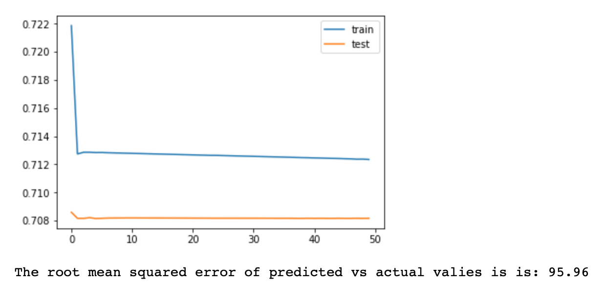
# The root mean squared error is the highest among all models: 95.96 compared to 24 in complex model and 23 in simple model
# Thus the preffered model is the single LSTM and Dense layer with t-1 pollution and other relevant variables as an input

# The training loss and valuation loss converge very fast to it's final outcomes
# Both loss and valuation loss are relatively high, about 0.70 level
# This means that this neural network is not efficient for time series prediction
# Compared to the complex model 2, it has worse outcome
# This model basically predicts that the pollution is equal to its mean over time

# The reason for worse performance of this model is that it apperars that t-1 predictions are the most relevant
# for predicting this time series at time t. This could be because the time series has very short memory, or because
# it is a markov chain (future given present is independent of past)

# Another possibility is that the network could be confused by too many variables (72*8 for each pollution record),
# thus it was harder to detect most relevant one